Environmental Effect on Wind Farm Efficiency and Power Production
Bennett Haskew 1, Liam Minogue 2, Reece Cohen Woodley 3, Adithep Phaktham 4, Shashikala Randunu 5.
University of Technology Sydney, Faculty of Science, P.O. Box 123, NSW 2007, Australia
1 Bennett.c.haskew@student.uts.edu.au
2 Liam.p.minogue@student.uts.edu.au
3 Reece.c.woodley@student.uts.edu.au
4 Adithep.phaktham-1@student.uts.edu.au
5 Upeksha.s.mirissalankage@student.uts.edu.au
Author to whom correspondence should be addressed; E-Mail: Bennett.c.haskew@student.uts.edu.au
DOI: http://dx.doi.org/10.5130/pamr.v3i0.1412
Abstract:
A meta-study is conducted investigating the effect of wind farm and turbine sites on the thermodynamic factors that affect energy production. Site deviations in surface roughness length, diurnal temperature changes of turbine and generation density and thermally stratified wind distributions are the parameters considered. The environment should be a significant factor in the placement of new wind farm sites. Further it is shown that with increasing wind velocity distributions negatively impacts efficiency of the turbine system and power output is decreased.
Keywords: Diurnal Temperature; Efficiency; Exergy; Surface Roughness Length; Thermal Stratification; Wake effect; Wind Shear Coefficient.
Nomenclature:
| SLR | Surface Length Roughness |
| ABL | Atmospheric Boundary Layer |
| WSC | Wind Shear Coefficient |
1. Introduction
The discussion of global energy consumption, greenhouse gas emissions and carbon footprint are at the forefront of today's societal consciousness. This places emphasis on the renewable energy sector, with energy systems being researched and implemented globally at an increasing rate. One such system is wind energy, which is one of the most renewable and energy efficient systems in the modern world [1]. Utilising this energy, wind turbine power generation systems have the potential for high efficiency, however they may have adverse environmental impact, and are dependent on that same environment for the best outcome as they convert the mechanical energy of the wind incident on the turbine blade into mechanical energy of the turbine to electrical energy in the generator. A thermodynamic analysis will find a relationship of energy and exergy to highlight the potential vs. actual power generated from a system and why this outcome occurs. The environment of the wind farm or individual turbine plays a major role in the success of that farm reaching its maximum generation potential to make an efficient system that is close to a purely adiabatic process. However, it is this same environment that may adversely affect the generational capacity of a farm and produce negative of suboptimal outcomes.
1.1 Working principles
The general working principle of wind power energy is based on the energy translation between mechanical energy and kinetic energy. The effective conversion of this energy is wind power output. Main features contributing to wind power output and the efficiency of this output include effective blade area, height of tower, geographical location and physical positon. A wind farm typically depends on the physical interaction of wind energy upon the wind turbine stream.
The most important meteorological resource assessed in many reports is wind speed. The Wind itself is the kinetic energy of the air in motion as molecules of gases in the atmosphere are constantly moving. The interaction of this kinetic energy on the blades of the turbine results in the rotation of the system giving mechanical energy. The rotors are perpendicular to the wind flow and air flow makes the rotors rotate around the hub. This energetic relation can be expressed in terms of volume, density and cross-sectional area perpendicular to the air flow. Wind energy can be related to kinetic energy as a flow of air mass to a velocity [2].
Figure 1 shows a wind turbine stream tube and the relationship between wind speed, atmosphere pressure, and temperature change and hub height. The variation in velocity, pressure and temperature are shown explicitly. Implicitly air density is a parameter of temperature and the transfer of mechanical energy is released as work done by the system in the form of heat.
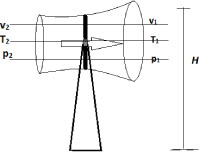
Figure 1: Schematic diagram of wind turbine stream tube.
2.0 Methods
This Meta study focuses on the thermodynamic environmental effects of and on wind farms and individual wind turbines. The literature ranged from papers published from 2003-2016 due to the availability of relevant data, that was retrieved from databases including the UTS Library, ScienceDirect and SCOPUS. Materials collected from government wind farm approval plans and direct manufacture specifications were used as well. The data collated in this study is presented Figures 2-9.
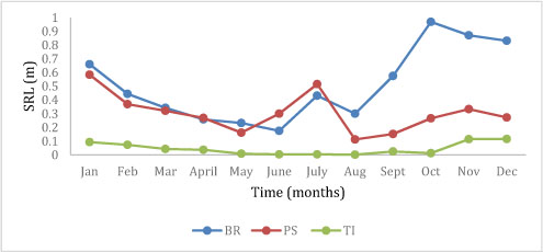
Figure 2. Shows the deviation of SRL over the course of a year across the three wind farms BR, PS and TI.
The three farms assessed in section 3.1 are all of costal locations in Southern Italy, Brindisi (BR), Portoscuso (PS), and Termini Imerese (TI). These were selected as they were an exhaustive scope of data accessible for this meta study. The farms assessed in 3.2 are also an exhaustive representation of accessible data on diurnal change in temperature because of windfarms, these were farms in the San Gorgino Gorge, California; Horns Rev, Denmark; Cedar Creek I, Iowa; CWEX, Iowa; Nolan County, Texas. In section 3.3 one farm was assessed for the wake effect of turbine placement. The two farms in the single study used were chosen to ensure consistency in this area because the parameter assessed is not the farm itself but the physical layout of the turbines with respect to individual cells. The single turbine assessment in 3.4 was selected because it was purposely made to produce a standardised model based on empirical data of wake effect in power production to ensure clarity.
The parameters invested are wind shear coefficient, site deviations in surface roughness length, turbine density and generation density, thermally stratified wind distributions and turbine placement in wake effect. Raw data from papers was used to produce graphs for Table 1 and Figures 2,3,5(L)-9. Raw data used to calculate new information was used in Figures 5R, 10 and 11.
The exergy efficiency parameters were unavailable for our purpose. The data presented for power produced (PProduced(kWh)) was in kilo-Watt-hours (kWh), we converted this to PProduced (kW) by equation (1), this raw data can been seen in Appendix A. Exergy efficiency was then calculated from the provided data of available power (Pavailable) in equation (2). The spread (range) of diurnal warming and cooling effects was calculated using equation (3).

3.0 Results and Discussion
3.1 Surface Roughness Length
Surface roughness is deviation from the normal vector of a surface in its ideal form, and is a direct representation of a surface's texture. A large deviation means the surface is rough, a small deviation is a smooth surface. Surface Roughness Length is similar parameter. It is not a physical length, but is a length-scale representation of a surface's ‘roughness’. It is the height at which wind speed theoretically becomes zero. Surface Roughness Length (SRL) is used in surface wind profile calculations, as part of larger studies assessing the output potential of an area for wind energy production. The Wind Shear Coefficient (WSC), also known as the wind shear gradient, is the difference in atmospheric wind speed over a short distance. For the purposes of wind turbines, difference in wind velocity over the blade of the turbine will demonstrate the energy that has been extracted from that wind by virtue of the change in kinetic energy. This coefficient is crucial in calculating the energy potential for an area but requires the calculation of a wind profile first [3].
Wind Profile calculations are used to assess the potential kinetic energy an area can provide, by acquiring an accurate velocity that takes into consideration the WSC and SRL (z0 in the literature). These variations are important as the output of the wind profile is then used to determine potential kinetic energy output for the region.
The following data was acquired from 3 costal monitoring stations in Sothern Italy, Brindisi (BR), Portoscuso (PS) and Termini Imerese (TI). The data was acquired by monitoring variations in wind at different heights, then using the above mentioned equations to first calculate the WSC, then using that to calculate the SRL. The monitoring stations raw data shows both monthly and diurnal trends when presented graphically. We reproduce two monthly graphs (Figure 2 and 3) from the tabulated data source[3].
Figure 2 shows drastic changes in the surface roughness, as would be expected from the changing sea levels. Additionally wind can dislodge dirt particulates which effect upward wind gradient as explained in Niu Qinghe,. Et al [4]. A comparison of Figure 2 and Figure 3 shows that over the same time span, the WSC changes in a similar trend to that of the surface roughness length. We make this trend more explicit by producing four further graphs that show the direct, seemingly linear relationships in Figure 4.
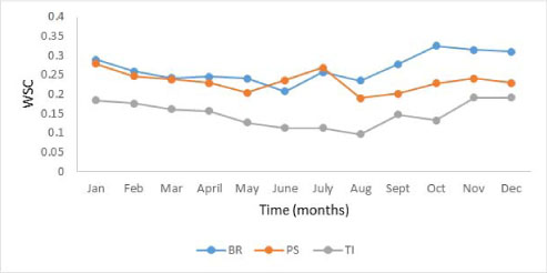
Figure 3. Shows the deviation in WSC over the course of a year across the three farms BR, PS, and TI.
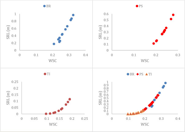
Figure 4: Top Left; SRL as a function of WSC at station BR showing a positive relation. Top Right; SLR as a function of WSC at station PS showing a positive relation. Bottom Left; SLR as a function of WSC at station TI showing a positive relation. Bottom Right; SLR as a function of WSC, showing the overall positive trend in the data.
From Figure 4 we can conclude there is a positive relationship between the WSC and the SRL such that with an increase in WSC there is a corresponding increase in SRL. This shows that the WSC has a direct impact on the calculated SRL used in the wind profile for a region. This conclusion can be extended to wind farms and their turbines, and that the potential kinetic energy that can be extracted is dependent on the SRL and the WSC. Further we can conclude that changes to the WSC are contributed to by thermal stratification and the effects wind farms have on surface temperatures, as when changes in the temperature of the ground occur, it creates a wind gradient in the surface air which in turn effects the WSC [4]. We recommendthat when new wind farms are been produced, planning teams should take into consideration these factors that affect the SRL and choose locations where the SRL remains stable at a higher level to produces a consistent level of power. Further studies into the effects surface air temperatures have on SRL would provide better tools for the assessment of wind farm locations, in order to obtain maximum power.
3.2 Effect on Surface Temperature from Wind Farms
Rajewsji et al. determined that there was both a diurnal warming and cooling effects down wind and up wind of wind farms respectively[5].This effect is causally related to the movement of the turbine blades in the atmospheric boundary layer (ABL). This turbulence, is thought to cause the temperature fluctuations [6]. In this section we evaluate the non-thermodynamic factors of average electrical generation density (MWkm-2) and average turbine density (km-2) and their effect of the relative diurnal cooling and warming effects. We assess the data from 5 wind farms San Gorgino Gorge, California [7]; Horns Rev, Denmark [1]; Cedar Creel I, Iowa [5]; CWEX, Iowa [6]; Nolan County, Texas [8]. These were chosen because they represented the only data sets available that assessed these warming and cooling effects and span studies that last from 4-25 years. Table 1 shows a summary of the wind farms we assessed.
3.2.1 Electrical Generation Density
Average Electrical generation density was assessed as a factor in both the warming and cooling effects detected in downwind and upwind areas of wind farms experienced in diurnal periods. We calculated the average electrical power output from the farms per unit area assessed and plotted them against the detected diurnal effects in Figure 5 these were produced using equation (3).
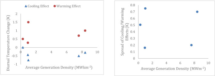
Figure 5. Diurnal warming and cooling effects on temperature as a function of average generation density for the five farms used in this meta study (left); Spread of Diurnal cooling/warming effects compared to the average generation density (right).
From Figure 5 there is no trend in the data presented, potentially more data in future studies may find a relationship between the diurnal temperature change and average generation density of the farm. However, given the current understanding of this thermodynamic phenomena; that it is caused by the mechanical motion of the wind turbine blades disrupting the ABL, rather than the tacit effect of generating an electrical current, this observation would be consistent with current literature [8]. We further assessed the range of the magnitude of the range between temperature changes relative to the average electrical generation density for each farm in Figure 5 right again, there seems to be no tend apparent in the range of the specific diurnal cooling/warming effects on any of our farms that were assessed, as a function of the energy density.
3.2.2 Turbine Density
The second non-thermodynamic factor of turbine density was investigated with regard to surface temperature of wind farms. We calculated the turbine density of each farm of turbines per unit area (km-2). The relationship between turbine density and diurnal surface warming and cooling can be seen in Figure 6.
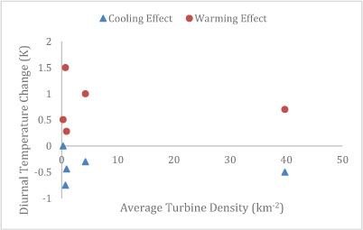
Figure 6. Dinural cooling and warming effects on temperature as a function of average turbine density.
Again either due to the limitations of data, there is no distinct relationship. Cooling/warming pairs of each farm appear to be clustered, however this is only because of the small data set used in this meta study. More studies may need to be conducted to fully assess this relationship.
It is important to note that this data is also affected by the minutia of the temperature changes recorded. The studies used for the purposes of this meta study were conducted of extremely long periods of time (3-25 years). During which time, the peak change in temperature on any given wind farm was 1.5 Kelvin, in Iowa in the CWEX study [8]. This may indicate there are a variety of other factors that may be influencing the relationship of turbine density and surface cooling and warming. We recommend Given that the presence of wind turbines and farms can materially affect the temperature of the microclimate surrounding the farm, firms should consider this factor when allocating a new wind farm site. Additionally, we recommend that further investigation be pursued in this area. Further all of the wind farms studied are on flat, grassy planes. It is plausible that different surfaces (ie, deserts, costal, inland) could produce less or more diurnal temperature effects. These are factors that should be considered in future, and investigated to determine an optimal wind farm site surface.
3.3 Thermal stratification
Thermal stratification is the process by which air is forced upwards due to thermal expansion and rise of air from the surface where temperatures are greater. This change results in decreasing net wind speed distribution [4,8].
Thermal stratification is strongly related to the wind shear coefficient by the effect of convection currents on surface roughness of wind [9]. We investigate this relationship by showing changes in hub height of wind turbines is a key component in overall performance. As a vertical component, which is typically changed due to variations of temperature and wind speeds at different heights, this can be interpreted as wind shear. However, as the accurate measurement of temperatures per small height increases is difficult and not presented in literature we have chosen to derive this temperature change by taking the wind speed at two vertical points see section 3.1 [6].
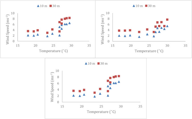
Figure 7. Average wind speed and temperature on a monthly basis at two evaluations on three different locations in south Pakistan. Top Left KatiBandar; Top Right Jati; Bottom Center Gharo. This data was chosen and graphed from tabulated data.
This study [9] investigated the influence of wind shear on the power production of a wind turbine focusing on the payback period and cost of energy for three coastal sites in southern Pakistan. As we see from the following graphs average temperature and elevation increases result in wind speed increases and are positively related. The change in available wind speed due to elevation caused by the dispersed effect of thermal stratification decreases change in vertical temperature variation and as temperature increase the expansion of air causes the greater wind speed [4,8].
3.4. Efficiency and Wake Effect
Performance of wind energy systems is dependent on topography, meteorological conditions and mechanical interactions, these parameters were explored in sections 3.1, 3.2 and 3.3 respectively. This section investigates what combinations of these parameters can have on a wind turbine power system. Exergy of a system is presented alongside efficiency, where exergy is a measure of maximum useful work that can be done by a system inclusive of its interaction with the environment [10]. This link means that exegetic analysis cannot distinguish absolutely between an environmental variable to system specific variables. However, this same argument links surface temperature, roughness and thermal stratification directly to the wind turbine system. Evidence of wind turbine systems effecting environmental conditions and therefore wind turbine output can be seen in the wake effect. Evidence of wake effect caused by a wind turbine is shown to affect wind speed and maximum useful work while, the variation of hub height and physical positioning is given as a contributing factor for turbine efficiency.
The efficiency of wind turbines depends on its model, specifications and wind speed [11]. Figure 8 shows the varied power outputs of three different turbines due to changes in wind speed. The meteorological resource highlighted is wind, described as the motion of large scale air masses with potential and kinetic energies [10]. This energetic relation can be expressed in terms of volume, density and cross-sectional area perpendicular to the air flow. Wind energy can be related to kinetic energy as a flow of air mass to a velocity [2]. The relationship of available kinetic energy from wind is used in previous sections to investigate how varied parameters can affect wind speed, however we will focus on standard wind speed in this section for simplicity. Figure 8 shows that given three different models higher wind speeds result in higher kinetic energy therefore a higher power output which is intuitively expected and supported by current literature. However, the interaction of this wind on the system does not show how much of the captured wind is actually converted into usable energy.
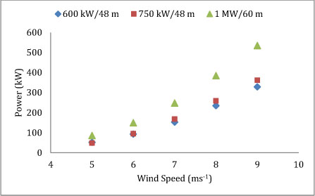
Figure 8. Power produced (kW) from three wind turbines for different wind speeds. Each category is given in nominal power/ rotor diameter. This data was chosen due to limited availability and proprietary pay gates that exceeded our limited resources [11].
The retardation of wind flowing through a wind turbine occurs in two stages. Knowing that the maximum work is extracted from a moving fluid when its velocity is brought to zero the kinetic energy and exergy of wind should be of equal value. However, the theoretical efficiency max given by Betz criterion is, 0.5926 approx. 60% [12]. Further, practical applications of wind turbines at optimal wind speeds usually attain up to 40% the rest of the wind energy is not obtainable and given as exegetic loss[9]
O. Baskut et al [10], present data from Nov 2007 to Sept 2008 on a wind turbine power plant of three turbines located in Germiyan-Cesme Turkey, model Enercon blade diameter 40m and nominal output 500kW. These turbines are numbered one to three corresponding to left to right respectively and physically positioned adjacent to each other but, have varied outputs. This specific system was chosen as Figure 8 shows the variations in power output given different models and it was decided that for consistency a standardized model should be used for clarity.
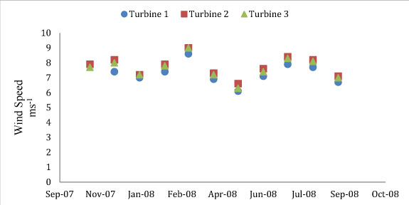
Figure 9. Shows the varied available wind speed to three equivalent turbines place next to each other against time. We have created this graph to visually show a relationship tabulated by a secondary source [10].
Constant environmental factors for all 3 turbines are recorded [10], yet, varied outputs are measured; we suggest that this is due to the wake effect as the turbines are numbered one to three representing left to right in physical placement, additionally the rotational direction of all three turbines is clock-wise. Between 6-7ms-1 wind-speeds, the variation in measured input can be linked to wake induced turbulence while at greater speeds, fluctuations in blade loading are shown to increase the overall stress a turbines mechanical components undergo therefore reducing efficiency due to fail safes [13]. We investigate wind speeds relationship further but do not explore mechanical components in this paper due to an inconsistency between available data and similar wind turbines models.
Expanding on the efficiency we show the amount of available energy used. We have taken the produced energy, derived from exergy efficiency and hours in operation, divided by recorded available power per month and plotted it against wind speed ms-1 to create Figure 10 [10], see equation (1).
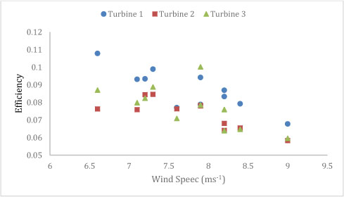
Figure 10. Shows the negative relationship between wind speed and efficiency. We produced this graph by deriving secondary data.
The efficiency against wind speed shows a negative trend as wind speed increases turbine output efficiency decreases. This supports the wake effect discussed in Figure 9 but also shows the difference between individual turbine efficiency. Turbine one on average maintains the highest efficiency while turbine two which had the highest average wind speed over time is shown to have the lowest efficiency. Variations in available wind speed on turbines that share the same environmental constants is shown and attributed to wake effect.
Physical position is shown to be a contributing factor to wind farm efficiency by individual turbines due to wake induced variations in outputs. This suggests that favorable variation of hub heights for large scale farms will increase overall output. A study provides computational data of the wind farm layout designs using varying distances between turbines and varying hub heights of each turbines [14]. We calculated efficiency by dividing recorded power output by available power to create Figure 11.
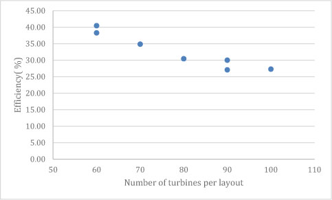
Figure 11. Calculated efficiency shows a negative relationship with larger turbine groups.
Chen, Y et al [14], explores the possibility in using different hub heights of wind turbines to generate more power output than wind turbines with the same hub height in the same limited area and is deemed successful; we support this conclusion by deriving the efficiency of their data in Figure 11. Expanding on this conclusion it is shown a greater distance between wind turbines is what improves performance the most, given the distance to allow the dispersion of wake, known as wake decay [13]. This is shown by a lower number of turbines in each layout providing a greater efficiency due to the placement of each turbine in a layout as wake effect is most prominent on turbines downwind [14].
Applying this finding to a large scale investigation has shown that efficiency can be optimised if turbines groupings are small and spaced far enough for wake to disperse; therefore, educated placement of wind farms is not only required to minimize negative environmental impacts but also to minimize detrimental factors of wind turbines on each other. Further, this evidence strongly suggests studies should be conducted on a case by case basis if an area is being surveyed for development to attain the most favorable conditions for firms.
4. Conclusion:
This paper has investigated the effect of wind turbines upon the land they occupy and also how placement of wind turbine farms can be optimized if properly assessed. The variables we have assessed are wind speed, temperature change, physical placement and model specifications. As the meta-analysis includes a broad spectrum of sources due to limited availability or relevance the relationships shown should be studied further for any future system development as it is shown environmental factors are key and specific to each location. This issue was overcome in part by using as many relevant data points as possible.
We observed not only a trend but a positive, linear relationship between SRL and WSC in costal wind farm locations. We observed that the WSC was affected by the SRL in a coastal environment due to the density of wind that would dislodge dirt particulates from the surface but, also the constant flowing of the ocean nearby would necessitate constant changing SRL given the WSC materially effects the kinetic energy that can be extracted from the site. It should be recognized that there will be variation in the power produced from a wind farm in a coastal location. It is plausible that wind farms in different environment for example planes or deserts would experience a different effect, this would be an area for future study.
We also saw no detectable relationship in the data provided between both the presence of and range between the diurnal warming and cooling effects with respect to both the turbine density and the generation density of planar farms. Further, we identified that with both higher temperatures and higher hub height the available wind speed incident on a turbine blade increased.
Physical position is shown to be a contributing factor to wind farm efficiency by individual turbines by a negative relationship between wind turbine efficiency as wind speed increases. Variations in available wind speed on turbines that share the same environmental constants is shown and attributed to wake effect. Further this evidence is applied to a large scale investigation showing that efficiency can be optimised if turbine groupings within cells are small and given sufficient distance to allow for wake decay. We conclude that the educated placement of wind farms is necessary to minimize negative environmental impacts, but, also detrimental factors of wind turbines acting upon each other.
The conclusions of this paper are limited in their validity due to limited access to data, and the presumption that the parameters assessed were an independent variable in any given paper. We recommend further studies into the parameters and areas assessed as dedicated studies rather than a meta study interpretation of secondary results. This is a critically important part of renewable energy science, not only given the imperative and importance of climate change in everyday societal thought, but also because of the environmental damage that may be caused as a function of wind farms. It should be noted that all of these facts may interlink; in some circumstances the increase in temperature which increases the wind speed may improve the overall performance of a farm, but this must counterbalanced against the exegetic efficiency that suffers as a result. Firms should strive to achieve the optimum equilibrium of these competing factors.
Acknowledgments
The authors would like to acknowledge the support and guidance of Jurgen Schulte from the University of Technology Sydney, Australia.
References
[1] Fitch, A., Lundquist, J. and Olson, J. 2013, Mesoscale Influences of Wind Farms throughout a Diurnal Cycle, Mon. Wea. Rev., vol 141, no 7, pp.2173-2198, doi: http://dx.doi.org/10.1175/MWR-D-12-00185.1
[2] Redha, A., Dincer, I. and Gadalla, M. 2011, Thermodynamic performance assessment of wind energy systems: An application, Energy, vol 36, no 7, pp.4002-4010, doi: http://dx.doi.org/10.1016/j.energy.2011.05.001
[3] Gualtieri, G. and Secci, S. 2011, Wind shear coefficients, roughness length and energy yield over coastal locations in Southern Italy, Renewable Energy, vol 36, no 3, pp.1081-1094, doi: http://dx.doi.org/10.1016/j.renene.2010.09.001
[4] Niu, Q., Qu, J., Zhang, K. and Liu, X. 2012, Thermodynamic effects on particle movement: Wind tunnel simulation results, Chin. Geogr. Sci., vol 22, no 2, pp.178-187, doi: http://dx.doi.org/10.1007/s11769-012-0526-0
[5] Harris, R., Zhou, L. and Xia, G. 2014, Satellite Observations of Wind Farm Impacts on Nocturnal Land Surface Temperature in Iowa, Remote Sensing, vol 6, no 12, pp.12234-12246, doi: http://dx.doi.org/10.3390/rs61212234
[6] Rajewski, D., Takle, E., Lundquist, J., Oncley, S., Prueger, J., Horst, T., Rhodes, M., Pfeiffer, R., Hatfield, J., Spoth, K. and Doorenbos, R. 2013, Crop Wind Energy Experiment (CWEX): Observations of Surface-Layer, Boundary Layer, and Mesoscale Interactions with a Wind Farm,Bull. Amer. Meteor. Soc., vol 94, no 5, pp.655-672, doi: http://dx.doi.org/10.1175/BAMS-D-11-00240.1
[7] Baidya Roy, S. and Traiteur, J. 2010, Impacts of wind farms on surface air temperatures, Proceedings of the National Academy of Sciences, vol 107, no 42, pp.17899-17904, doi: http://dx.doi.org/10.1073/pnas.1000493107
[8] Howard, K., Chamorro, L. and Guala, M. 2015, A Comparative Analysis on the Response of a Wind-Turbine Model to Atmospheric and Terrain Effects, Boundary-Layer Meteorol, vol 158, no 2, pp.229-255, doi: http://dx.doi.org/10.1007/s10546-015-0094-9
[9] Rehman, S., Shoaib, M., Siddiqui, I., Ahmed, F., Tanveer, M. and Jilani, S. 2015, Effect of Wind Shear Coefficient for the Vertical Extrapolation of Wind Speed Data and its Impact on the Viability of Wind Energy Project, Journal of Basic & Applied Sciences, vol 11, pp.90-100, doi: http://dx.doi.org/10.6000/1927-5129.2015.11.12
[10] Baskut, O., Ozgener, O. and Ozgener, L. 2011, Second law analysis of wind turbine power plants: Cesme, Izmir example, Energy, vol 36, no 5, pp.2535-2542, doi: http://dx.doi.org/10.1016/j.energy.2011.01.047
[11] Koroneos, C., Spachos, T. and Moussiopoulos, N. 2003, Exergy analysis of renewable energy sources,Renewable Energy, vol 28, no 2, pp.295-310, doi: http://dx.doi.org/10.1016/S0960-1481(01)00125-2
[12] Ozgener, O., Ozgener, L. and Dincer, I. 2009, Analysis of Some Exergoeconomic Parameters of Small Wind Turbine System, International Journal of Green Energy, vol 6, no 1, pp.42-56, doi: http://dx.doi.org/10.1080/15435070802701777
[13] Storey, R., Cater, J. and Norris, S. 2016, Large eddy simulation of turbine loading and performance in a wind farm, Renewable Energy, vol 95, pp.31-42, doi: http://dx.doi.org/10.1016/j.renene.2016.03.067
[14] Chen, Y., Li, H., Jin, K. and Elkassabgi, Y. 2015, Investigating the possibility of using different hub height wind turbines in a wind farm, International Journal of Sustainable Energy, pp.1-9, doi: http://dx.doi.org/10.1080/14786451.2015.1007139
5. Appendix
5.1 Appendix A
| Turbine 1 | ||
| Power Produced (kWh) | Hours | Power Produced (kW) |
| 127973 | 563 | 227 |
| 92775 | 471 | 197 |
| 122896 | 654 | 188 |
| 116661 | 524 | 223 |
| 168376 | 662 | 254 |
| 114976 | 612 | 188 |
| 76502 | 632 | 121 |
| 102236 | 624 | 164 |
| 151661 | 664 | 228 |
| 133514 | 656 | 204 |
| 94130 | 594 | 158 |
| Turbine 2 | ||
| Power Produced (kWh) | Hours | Power Produced (kW) |
| 133151 | 592 | 225 |
| 140439 | 649 | 216 |
| 116099 | 631 | 184 |
| 116654 | 517 | 226 |
| 172904 | 675 | 256 |
| 117660 | 620 | 190 |
| 82727 | 659 | 126 |
| 111911 | 664 | 169 |
| 153784 | 671 | 229 |
| 142264 | 698 | 204 |
| 96668 | 599 | 161 |
| Turbine 3 | ||
| Power Produced (kWh) | Hours | Power Produced (kW) |
| 141049 | 601 | 235 |
| 151368 | 677 | 224 |
| 115958 | 646 | 180 |
| 108279 | 503 | 215 |
| 181894 | 695 | 262 |
| 121653 | 629 | 193 |
| 84053 | 659 | 128 |
| 105206 | 628 | 168 |
| 142473 | 671 | 212 |
| 135520 | 697 | 194 |
| 91249 | 568 | 161 |
![]()
©2016 by the authors. This article is distributed under the terms and conditions of the Creative Commons Attribution 4.0 International License (http://creativecommons.org/licenses/by/4.0/).