Construction Economics and Building

Vol. 25, No. 2
July 2025

RESEARCH ARTICLE

A Methodological Framework to Assess the Employment Impacts of Transport Infrastructure Construction

Heikki Savikko^1,2,*, Joonas Hokkanen², Heikki Metsäranta², Juha Honkatukia³, Mika Haapanen⁴, Timo Tohmo⁴, Eva Pongracz¹

¹ University of Oulu, P.O.Box 8000, FI-90014 University of Oulu, Finland

² Ramboll Finland Oy, Kansikatu 5B, 33100 Tampere, Finland

³ Merit Economics, Ristiretkeläistenkatu 16 A 3, 00710 Helsinki, Finland

⁴ Jyväskylä University School of Business and Economics, P.O. Box 35, FI-40014 University of Jyväskylä, Finland

Corresponding author: Heikki Savikko, heikki.savikko@student.oulu.fi

DOI: https://doi.org/10.5130/AJCEB.v25i2.8894

Article History: Received 02/11/2023; Revised 13/11/2024; Accepted 07/04/2025; Published 08/08/2025

Citation: Savikko, H., Hokkanen, J., Metsäranta, H., Honkatukia, J., Haapanen, M., Tohmo, T., Pongracz, E. 2025. A Methodological Framework to Assess the Employment Impacts of Transport Infrastructure Construction. Construction Economics and Building, 25:2, 143–167. https://doi.org/10.5130/AJCEB.v25i2.8894

Abstract

The aim of this study was to suggest a methodological evaluation framework for assessing the employment impacts of transport infrastructure construction. The applicability and usability of different ex-ante employment impact assessment methods were evaluated. Commonly, the employment impacts during construction are used as a justification for investment decisions. In this study, we tested three commonly used methods to estimate the employment impacts during the construction of three real-life case studies and compared the results to the known impacts of these projects. The results indicate that transport infrastructure construction is not an effective means of employment policy nationwide. This is partly due to insufficient labor supply in the infrastructure engineering and construction industries. A higher employment rate on a national level would require an increase in labor supply instead of an increase in labor demand. However, even though the national net impact on employment was close to zero, the gross regional impact on employment would still be useful information in project planning. The methodological framework, presented in this paper, helps to manage the employment impacts of transport infrastructure construction in a proper context.

JEL classification

L74 Construction; J23 Labor Demand; J21 Labor Force and Employment, Size, and Structure; C67 Input–Output Models; C68 Computable General Equilibrium Models

Keywords

Infrastructure Construction; Impact Assessment; Employment Effects; Employment Policy; Employment Evaluation Framework

Introduction

Transport infrastructure enables accessibility, which is a vital function in a society. Infrastructure projects are often justified based on their direct, indirect, and induced gross employment effects during construction, and have traditionally been seen as good economic policy tools. However, in the European Commission’s Guidelines for the Cost-Benefit Analysis of Investments Projects (2014), labor during construction is considered a cost, not a benefit. There are also different methods to evaluate employment impacts during construction, but the topic has received relatively little attention in the literature, which tends to focus on post-construction impacts (Purwanto et al. 2017; Laird and Venables, 2017, de Rus et al., 2022) and gross changes, i.e., the jobs created or saved (Wilson, 2012), or has used methods not suitable for ex-ante evaluations (Garin, 2019; Alloza and Sanz, 2021).

In this study, we examine the gross and net employment effects during construction of transport infrastructure and their relationship to economic and industry cyclical conditions and transport project characteristics. This is done by using three commonly used ex-ante evaluation methods: labor input coefficients, static input–output (IO) model, and computable general equilibrium (CGE) model. The methods are demonstrated on three real-life cases: a railway project, a highway project, and a road investment program. After the ex-ante assessment, we compare the results to the known impacts of the three projects. Ultimately, we outline a methodological framework for selecting suitable ex-ante evaluation methods to assess the employment impacts of transport infrastructure investments during construction. By employment impact, we refer to the change in employment caused by the project or other measure under assessment, measured in terms of the number of people employed or the number of person-years of work. Gross change in employment refers to the demand for labor generated directly or indirectly by the project, without considering whether the labor required comes from outside the existing workforce, for example, from the unemployed or students, or whether it is a shift from other jobs. The net employment impact refers to the change in the employment rate in the economy.

The study focuses only on the construction period, and pays no attention to the employment impact of transport system efficiency and accessibility improvements. The main finding is that the type of information needed on employment impacts determines the selection of assessment tool. If information is needed to help the timing of projects in different regions, or to examine the demand for labor and skills in the future, labor input coefficients and input–output models are suitable methods. If we need to determine the net employment effects on a regional or national level, a computable general equilibrium model is the most suitable method. However, it will require an assessment of the labor market situation and labor supply before modeling. Based on the results of this study, we also recommend that the assessment of labor needs is to be added to the project appraisal of transport infrastructure investments, to provide a more detailed analysis of the cost estimate. By considering project-specific data needs, the methodological framework proposed by this study aims to save time and costs while effectively allocating valuable resources in the project development phase.

The rest of the study is organized as follows: The next section is the review of relevant literature. Materials and Methods describes the used evaluation methods and the three cases. Under this section, the evaluation of the case studies using the three methods and the uncertainty related to employment impacts and economic cyclical trends are also covered. Next, we have the Results and Discussion sections, which also describes the suggested methodological framework. Lastly, the final section provides the conclusions. The study was commissioned by the Prime Minister’s Office of Finland.

Literature review

Research on the employment effects of transport infrastructure projects during the construction phase is limited, and impact assessments are rare in practice, even for nationally significant projects (Wang, 2015). Recent studies have focused on methods that are not directly applicable to ex-ante evaluations, or on impacts based on transport system efficiency and accessibility improvements. In the existing literature on ex-ante assessments of transport infrastructure construction, there is also often a lack of distinction between gross and net employment effects, which entails the risk of confusing the effort required with the benefits that will be accrued because of the project.

Garin (2019) utilized the difference-in-difference (DiD) method to analyze the impacts of a $27 billion highway infrastructure project in the United States. The study found that while construction activities positively affected direct employment in the local construction sector, net employment effects were nearly zero both regionally and locally. Notably, the construction of transportation infrastructure did not displace local labor from other construction activities, suggesting that the direct workforce was drawn from other sectors rather than a construction sector.

Similarly, Alloza and Sanz (2021) employed the DiD evaluation method to assess the impacts of Spain’s economic and employment recovery plan, which allocated approximately €13 billion to public investments at the municipal level. Their findings indicate that the recovery program generated 5.2 jobs per million euros invested, 8 months after the demand shock, with cumulative unemployment reductions of 6.5 person-years per million euros over 2 years. Based on that, the net effects were 1.25 times greater than the gross effects. The DiD method used by Garin, as well as Alloza and Sanz, is not suitable for ex-ante evaluations, but based on the results of their studies; it is possible to develop labor input coefficients for similar projects.

Dimitriou and Sartzetaki (2022) evaluated the socioeconomic impacts of a new regional airport in Greece using IO framework. Over the 5-year construction period, one direct job supports 1.0 job in other sectors. In a similar vein, Pienaar (2024) applied an IO model to assess the impact of rural road provision on employment in South Africa, finding that one direct job created during construction supports 2.3 jobs in the country. Lieuw-Kie-Song et al. (2019) analyzed the employment impacts of public expenditure on different types of infrastructure in Rwanda’s construction sector using established multiplier analysis combined with an employment satellite account. They concluded that most of the additional employment created is within the construction sector itself, and on average, one job in the construction sector creates another job in other industries.

All three ex-ante studies focused solely on gross employment effects, neglecting net employment impacts although Lieuw-Kie-Song et al. suggested that additional employment sometimes manifests as an increase in total working hours rather than changes in employment or unemployment rates. Dimitriou and Sartzetaki also seem to have confused the efforts required with the benefits that will be accrued from the project in their policy recommendations.

Langston and Crowley (2021) measured the success of the Gold Coast Light Rail (GLCR) transport infrastructure project stages 1 and 2. Their approach to facilitating decision-making in ex-ante evaluations involves the i3d3 model, a modern form of multi-criteria decision-making (MCDM). This model allows for the comparative assessment of various projects, ranking them from best to worst alternatives. Their approach serves as a valuable addition to traditional evaluation models, where technical expertise is essential. They also highlight challenges associated with traditional evaluation methods, noting that these processes are time-consuming, expensive, and open to manipulation. Their findings indicate a need for concrete frameworks for traditional evaluation methods to clarify assessments.

The need to clarify the use of different evaluation methods also arises from the Teo et al. (2022) study, where they reviewed economic impact assessment methods adopted in construction-related projects. They noted that most economic analyses are based on IO tables, even when the focus is on a specific sector, industry, or local region. They suggested that utilizing a detailed cost breakdown of projects and using multipliers to estimate impacts could provide more accurate assessments if the point of view is micro-level.

Based on the existing scientific literature, there is no clear consensus on which evaluation methods should be used when assessing ex-ante employment impacts during construction. Different methods have their own benefits, applications, and limitations, which should be considered when selecting the method to be used. This study aims to narrow this research gap by outlining a methodological framework for selecting suitable ex-ante evaluation methods to assess the employment effects of transport infrastructure investments during construction.

Materials and methods

International evaluation guidelines regularly analyze the employment impacts of construction as follows (Ernst and Marianela, 2015; Moszoro, 2021; World Bank, 2021):

1. Direct employment: Construction, design, or other work for a contractor or sub-contractor on a project.

2. Indirect employment: Work done in the production of intermediate products for construction. The impact is spread across a range of industries, typically in sectors such as construction equipment and transport services.

3. Induced employment: The increase in consumption resulting from the additional income of the people directly and indirectly employed by the project will further increase the demand for goods and services in different sectors.

4. Net employment: The change in the employment rate in the economy brought by the project, considering the crowding out effect of additional labor demand on the existing labor force and employment developments in the absence of the project being evaluated.

In the case studies carried out in this study, the employment effects were examined according to the same classifications using labor input coefficients, the static input–output model, and the computable general equilibrium model.

Input–output models

Static input–output (IO) models describe the structure of the economy at a given point in time as a cross-section over 1 year. Using input–output model to evaluate employment impacts, the results can be examined by industry and, depending on the model, sometimes also broken down by regions if the used model is a multi-region static input–output model (MRIO model). The MRIO model is an extension of the traditional IO model and considers the production structures of different regions and the trade flows between them. The inclusion of regional specificities in the model makes it a useful tool for testing national measures and regional economic resilience (Anagnostou and Gajewski, 2021). The interdependencies between sectors and the coefficients describing them are fixed in IO models, so that the economy is examined based on different scenarios (Miller and Blair, 2009).

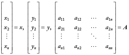
In an IO context, the economy is divided into n number of industries. If total output in industry i is given as x_i and final demand for industry i is given as y_i, a simple equation can be written to show how the products of industry i are distributed to other industries and to final consumption (Miller and Blair, 2009).

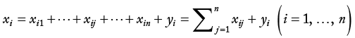(1)

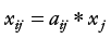
In the equation, the term x_ij describes the intermediate consumption of industries between industries and y_i denotes the final consumption of industry i. The input coefficients can be calculated from the input–output table:

(2)

The input coefficient a_ij expresses how much output is needed in industry j to produce one unit of output in industry i. The production model can now be constructed by substituting the input equation for intermediate demand into the balance equation (1)

(3)

obtained from the definition of the input coefficients (2). The production model is:

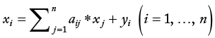(4)

and in models that have a regional extension (MRIO models), industries are considered by region g and the production model can be represented as (Leontief and Strout, 1963):

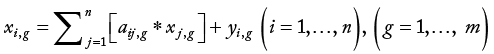(5)

The production model is:

when matrix entries are used

The production model has as many linear equations as there are variables to solve. The output of industries can be calculated separately in terms of the known demand for final products at any given time and region. However, it is more appropriate to calculate the equation group

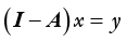(6)

a general solution:

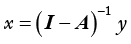(7)

Then, employment (L) is obtained by the formula (Markaki and Belegri-Roboli, 2010):

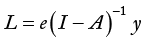,(8)

where e is the industry-specific direct labor input coefficient.

The static IO model used in this study was an MRIO model, where the model describes the economic activity in Finland and the interactions between different actors. The model was based on the NUTS-2 (Nomenclature of Territorial Units for Statistics) classification system of the European Union of five large areas of Finland, and it is a regionalized extension from the Finnish IO tables provided by Statistics Finland (OFS, 2021a). Regionalization based on existing statistics and using location quotients has been described in our previous works (Savikko, 2014; Hokkanen et al., 2017; Savikko et al., 2021).

Using the IO model gives a picture of the distribution of employment across industries and regions. This is possible by considering the increase in consumption resulting from the change in the earned income of those employed and the employment it continues to generate (Miller and Blair, 2009). Therefore, induced employment can be estimated as an increased consumer demand in different industries using the same formulas as presented previously.

Labor input coefficients

The labor input coefficient determines the number of person-years or person-hours spent per input produced in different industries. Labor input coefficients distinguish between direct impacts and total impacts. Direct impacts refer to the use of labor input in the sector concerned. Total impacts also include the use of labor input in the production of intermediate goods in other sectors serving the industry under consideration, but the results cannot be examined by industries. The labor input coefficients also do not consider the increase in consumption resulting from the change in the earned income of those employed and the employment that it continues to generate.

Using labor input coefficients, the direct employment (L_i) on industry i is:

,(9)

and total employment (L) can be presented as:

,(10)

where e_direct,i is the industry-specific direct labor input coefficient and e_tot,i is the industry-specific total labor input coefficient.

For this study, the labor input coefficients were based on the coefficient for the year of project implementation and were obtained directly from Finland’s national input–output statistics (OSF, 2021a).

Computable general equilibrium models

Computable general equilibrium (CGE) models describe the economy in terms of decisions taken by households, firms in different sectors, and the public sector. Consumption and saving decisions and labor supply are key household decisions. These decisions are described in national economic models based on historical consumption patterns, which also consider the evolution of relative commodity prices and household disposable income. Firms decide on the use of inputs—labor, capital, and intermediate inputs—to maximize the margin of production and investment according to the evolution of profit expectations in different industries relative to their historical growth rate and rate of return on capital. The functioning of the public sector is mainly determined by the structure of taxation and the transfers of income to households and other public actors. Foreign countries are mainly considered from the perspective of exports and imports, but the evolution of the external debt and wealth of the economy is also monitored and, in the long run, the external balance becomes dominant in the equations of the model. In CGE models, supply and demand are balanced through price mechanisms.

When the CGE model calculates scenarios of future development prospects, many of the key drivers of economic growth are defined outside the model, and the model’s task is then to calculate scenarios for the development of economic factors that depend on these external factors. For Finland, the modeling assumptions for economic growth come from outside the model from Statistics Finland’s population projections. In the CGE model, economic theory provides the framework within which history is interpreted, and economic trends and projected population growth derived from history provide the framework within which economic agents make their decisions.

In this study, computable general equilibrium modeling was performed using the FINAGE/REFINAGE model (Honkatukia et al., 2019), which has been developed from the VATTAGE (Honkatukia, 2009) and VERM models (Honkatukia, 2013). The model relates labor market equations to the population and the working age population, from which unemployment rates are determined based on labor supply and demand. The FINAGE/REFINAGE model operates on NUTS 3 level, where Finland is divided into 19 regions.

In dynamic simulations, labor supply comes as an exogenous variable, while wages adjust gradually, and unemployment is determined endogenously. The basic structure of the Anonymous 1 model is based on the idea that wages can be centralized at the national level, since in a dynamic environment, the adjustment of real wages is a slow element. The model assumes that real after-tax wages change slowly in the short run and are flexible in the long run. In this labor market specification, new shocks cause short-term changes in total employment and long-term changes in real wages. Algebraically, it is assumed that:

,(11)

where old is the predictive value of the base case. Wt,_old and Et,_old are the real wage and employment rate in year t in the base case projections and W_t and E_t are the real wage and employment rate in year t in the shock simulation. According to this definition, real wage adjustment depends on deviations from expected real wage growth and employment deviations from expected employment growth. The rate of adjustment is controlled by parameter α₁, while α₂ determines whether employment returns to the expected growth path after the shock. The real wage equation is close to the NAIRU unemployment theories (Dixon and Jorgenson, 2012), and its parameters for Finland have been estimated from previous studies as Alho (2002) and McMorrow and Roeger (2000).

Cases

We tested the previously presented evaluation methods to estimate the employment impacts during the construction in three real-life project and compared the results to the known impacts of these projects. Since the aim of the study was to outline a methodological framework for selecting suitable ex-ante evaluation methods to assess the employment effects of transport infrastructure investments during construction, we compared different cases, in terms of their size and type, to illustrate the applicability of different evaluation methods.

In the evaluation of employment impacts using labor input coefficients, the employment impacts were derived by multiplying the investment by the labor input coefficient of the construction industry. Labor input coefficients included separate values for direct impacts and total impacts that included direct and indirect employment impacts. It was assumed that the investment would be fully allocated to the construction industry.

When evaluating employment impacts using the IO model, it was also assumed that the investment would be fully allocated to the construction industry. The cost corresponding to the investment was allocated as new demand to the construction industry of the region or regions under review. Based on the IO model, direct and indirect employment impacts were evaluated. The IO model also accounts for changes in wages, which were used to calculate induced employment effects. Changes in wages of employees working on value chain of construction industry were distributed as new demand across various industries and savings based on household consumption statistics. After that, induced employment impacts were evaluated similar to direct and indirect employment impacts.

In the CGE model, the evaluation of employment impacts differs from the other methods. The investments of the evaluated projects are directly allocated to the investments in the industry responsible for transport infrastructure, with their costs reflected in the government’s budget. Employment impacts are determined through the labor demand of industries producing transport investments, as the investment levels change, and a new equilibrium is calculated for the economy. The employment impacts are compared to the actual development, under the assumption that the case projects would not have been realized. The difference in employment is the net employment effect. Direct employment impacts were estimated by assuming that the employment impacts in the construction industry within the investment region are direct impacts.

The key indicators of the three cases have been summarized in Table 1.

**Table 1. Information concerning the data cases.**
	Case 1	Case 2	Case 3
Country	Finland	Finland	Finland
Investment	€74.60 million	€21.35 million	€325.00 million
Region of direct impacts at NUTS 3 level	Central Finland and Pirkanmaa (see Figure 1)	Northern Ostrobothnia (see Figure 2)	Whole Finland (see Figure 3)
Time period of data	2015–2017	2015–2017	2016–2018
Data source	Finnish Transport Infrastructure Agency, 2017	Finnish Transport Infrastructure Agency, 2021	Finnish Transport Agency, 2017

Case 1: Äänekoski railway project. In the Äänekoski project, the railway connections in Central Finland were overhauled to meet the increased transport needs resulting from the investment in a new biofuel plant. The railway project was implemented under an alliance model, with the Finnish Transport Infrastructure Agency as the contracting party and VR Track Oy as the service provider. The project started in October 2015 and was completed in August 2017 (Finnish Transport Infrastructure Agency, 2017). The main work phases of the project included electrification of the Jyväskylä–Äänekoski section, replacement of the track superstructure, improvement of drainage, improvement of safety at level crossings, and renovation of the Kangasvuori tunnel. Geographical location of the Äänekoski railway project is presented in Figure 1. The project was implemented at a total cost of €74.6 million.

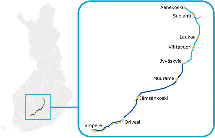
Figure 1. Geographical location of case 1: the Äänekoski railway project (modified from Finnish Transport Infrastructure Agency, 2017).

Case 2: highway 8 between Pyhäjoki and Liminka. Between 2015 and 2018, highway 8 was improved in several places between Himanka, Pyhäjoki, and Liminka (Figure 2). The main content of the project was the construction of a road connection to the area of the planned nuclear power plant in Pyhäjoki and the improvement of traffic capacity and traffic safety on the Kalajoki-Liminka section of highway 8. The Finnish Parliament decided to fund the project in spring 2015, and the construction work was carried out between 2015 and 2017. The cost estimate of the project package estimated here was €21.35 million (ELY Centre, 2015; Finnish Transport Infrastructure Agency 2021).

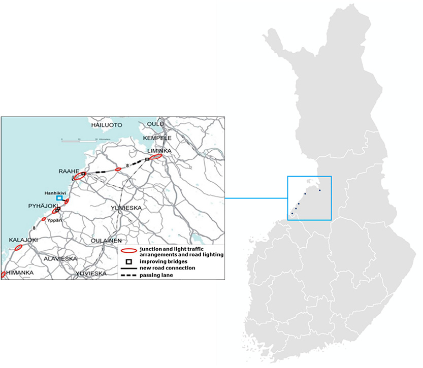
Figure 2. Geographical location of case 2: highway 8 between Pyhäjoki and Liminka (modified from Finnish Transport Infrastructure Agency, 2021).

Case 3: Road repair debt program 2016–2018. The road repair debt program 2016–2018 was a road investment program implemented with additional funding of €595 million granted by the Government to the Finnish Transport Agency (Finnish Transport Agency, 2017). The program consisted mainly of road, rail, and waterway rehabilitation projects, the aim of which was to halt the deterioration of the roads and the increase in the repair debt. The repair debt is the amount of money needed to bring the state’s roads, railways, and waterways up to current standards. The program also funded, for example, the development of a digital road infrastructure and a test site for automated traffic in Lapland. The case evaluation considered the repair debt program projects on the road network, which was €325 million (Figure 3).

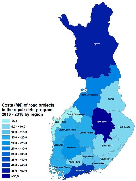
Figure 3. Costs of road projects by region in case 3: Repair debt program 2016–2018.

Results

From the cases, gross labor input requirements were estimated using the previously described labor input coefficients, the IO model, and the CGE model. The net employment effects were estimated using a CGE model with two different assumptions—with regional and national labor markets. This modeling approach enables comparisons of the meaning of the initial data and assumptions needed in modeling.

By analyzing the model-specific results of the different case projects and comparing the results with each other and with the reported project results, the advantages and limitations of the different evaluation methods were identified. The analyses were used to define a theoretical and methodological framework for assessing the employment effects of transport infrastructure investments during construction.

Case 1: Äänekoski railway project

The Äänekoski railway project was implemented as an alliance project, and therefore, it was reported more comprehensively than a basic project in terms of the need for labor. The final report of the project, published by the Finnish Transport Infrastructure Agency (2017), states that the number of staff, at approximately 170, remained stable throughout the project. The project trained 1,230 people and 539,452 person-hours were worked by the end of the implementation phase alliance agreement. The data in the final project report can be derived in person-years by using the duration of the project and the average number of staff. The duration of the chipping was 22 months, with a direct employment impact of around 312 person-years based on the average number of people employed.

However, the actual project data only reflect direct impacts and do not consider the indirect, induced, or net employment impacts that arise through other channels in addition to the direct impacts. Table 2 shows the data on the employment impacts of the Äänekoski railway project obtained by different evaluation methods.

**Table 2. Actual data on the Äänekoski project and the employment impact (in terms of person-years) obtained by different evaluation methods. The reference period is approximately 2 years.**
Äänekoski railway project	Actual	Labor input coefficients	Static IO	CGE, regional labor market	CGE, national labor market
Direct employment	312	469	379	384	387
Indirect employment	Not known	405	484	Cannot be presented	Cannot be presented
Induced employment	Not known	Cannot be counted	234	Cannot be presented	Cannot be presented
Net employment	Not known	Requires separate assessment	Requires separate assessment	631	−151

Evaluated direct employment impacts are greater than the actual impacts in all assessment methods, with overestimations ranging from 21% to 50%, depending on the assessment method. Actual indirect, induced, or net employment effects are not known, but when comparing the indirect employment impacts calculated with labor input coefficients and with the IO model, the indirect employment impacts are higher when evaluated using the IO model compared to labor input coefficients. However, the sum of direct and indirect employment impacts differs only by 1%.

With the IO model, it was also possible to capture the multiplier effects of consumption, induced employment, which were approximately 75% of the actual direct employment impacts. However, the IO model does not consider the crowding out effect, and all employment effects are gross effects.

When modeling with the CGE model, it is significant what is assumed about the labor markets. The net employment effects vary significantly based on labor market assumptions, ranging from more than double the actual direct impacts to nearly 0.5 times negative. If the availability of labor is assumed to be mainly regional, the effects will mainly be on the provinces of Central Finland and Pirkanmaa. In this case, changes in labor demand are mainly reflected in the regional employment rate. If, however, the labor market is national, migration balances the effects. With a regional labor market assumption, the effects will mainly be in the construction and trade sectors but, if the labor market is national, with migration, the effects will also be more on the processing industries. The labor market is always case- and region-specific and should be evaluated before modeling with a CGE model.

Case 2: highway 8 between Pyhäjoki and Liminka

For the project on highway 8 between Pyhäjoki and Liminka, there were performance data for six different contract areas (A–F), for all of which the costs (€) and working hours (h) per contract area were reported separately. The actual data also included person-years worked by region based on hours worked, as well as labor input coefficients (Table 3).

**Table 3. Actual data on direct impacts by project area. Period under examination: 3 years.**
Project area	Cost, €	Hours worked, h	Person-years	Labor input coefficient
A	1,276,617	9,970	6	4.9
B	10,670,528	92,979	58	5.4
C	1,804,842	17,670	11	6.1
D	206,000	700	0	2.1
E	5,069,647	46,420	29	5.7
F	2,321,250	29,806	19	8.0
Total	21,348,884	197,545	123	5.8

By comparing the project’s actual direct employment impacts with the results obtained using different evaluation methods, the direct impacts estimated using the labor input coefficients and the IO model are very close to the reported actual impacts, only 5% higher. The impacts estimated using the CGE model focus mainly on net employment impacts, and the direct gross employment impacts derived from the modeling results differ from the other evaluation methods. Direct employment impact evaluated with the CGE model was 68 jobs in both regional and national labor market situations, which is only 55% of actual impacts (Table 4).

Table 4. Actual data on Highway 8 between the Pyhäjoki and Liminka project and the employment impact (in terms of person-years) obtained by different evaluation methods. Period under examination: 3 years.
Highway 8 between Pyhäjoki and Liminka	Actual	Labor input coefficients	Static IO	CGE, regional labor market	CGE, national labor market
Direct employment	123	129	129	68	68
Indirect employment	Not known	111	137	Cannot be presented	Cannot be presented
Induced employment	Not known	Cannot be counted	69	Cannot be presented	Cannot be presented
Net employment	Not known	Requires separate assessment	Requires separate assessment	88	−50

In the CGE model, evaluated change is allocated to investments, and the effects on employment are determined through the labor demand of industries producing transport infrastructure investments. In Northern Ostrobothnia, the share of construction in road maintenance investments in the public sector is higher than the average for the entire country, so the direct employment impacts appear to be smaller than realized.

Comparing the indirect employment impacts calculated with labor input coefficients and with the IO model, the sum of direct and indirect employment impacts differs by 10%, being estimated higher by the IO model. Induced employment effects were approximately 56% of the actual direct employment impacts.

The net employment effects vary based on labor market assumptions, ranging from 0.7 to 0.4 times negative from the actual direct employment impacts. If the labor market is assumed to be national, the effects at the level of the entire country would have been negative, as the project would have displaced labor from the growth centers of Southern Finland.

Case 3: Road repair debt program 2016–2018

There is no measured and reported performance data on the road repair debt program. However, when estimated using different evaluation methods, the direct gross employment impacts are all the same order of magnitude, and the modeling results are quite close to each other (Table 5).

**Table 5. Actual data on the road repair debt program and the employment impact (in terms of person-years) obtained using different evaluation methods. Period under examination: 3 years.**
Road repair debt program 2016–2018	Actual	Labor input Coefficients	Static IO	CGE regional labor market	CGE national labor market
Direct employment	Not known	1,870	1,738	1,603	1,661
Indirect employment	Not known	1,633	2,026	Cannot be presented	Cannot be presented
Induced employment	Not known	Cannot be counted	1,012	Cannot be presented	Cannot be presented
Net employment	Not known	Requires separate assessment	Requires separate assessment	1,918	−26

Comparing employment impacts evaluated with different evaluation methods, the highest direct employment impacts were calculated with labor input coefficients in cases 1 and 2. Direct employment impacts evaluated with the IO model were 93%, with the CGE model using regional labor market assumption 89%, and the CGE model using national labor market assumption 89% of the highest direct employment impacts evaluated by labor input coefficients.

Comparing the indirect employment impacts calculated with labor input coefficients and with the IO model, the sum of direct and indirect employment impacts differs by 7%, with that estimated by the IO model being higher. Induced employment effects were approximately 58% of the direct employment impacts evaluated with the IO model. The net employment effects vary based on labor market assumptions, ranging from 1.1 to 0.02 times negative from the direct employment impacts evaluated with the IO model.

The third case differs from the first two cases because it was aimed at all regions in Finland and, by default, the implementation of the repair debt program has taken place nationwide. The biggest employment effects on all regions come from the construction industries. If the labor markets were regional, the effects would be almost entirely positive and higher than in the case of the national labor market. In the case of the national labor market, many other industries suffer because resources have been committed to construction and the net employment effects are close to zero.

Uncertainty related to employment impacts and economic cyclical trends

For all the evaluation methods used, the employment effects depend essentially on the sector-specific labor input coefficients [see equation (8)]. The values of direct labor input coefficients have fluctuated in recent decades (Table 6). In Finland, labor input coefficients in construction have ranged between 5.50 and 6.45 between 2000 and 2018. Similarly, they have varied between 5.86 (2018) and 7.72 (2002) in Central Finland and between 5.03 (2018) and 6.97 (2002) in North Ostrobothnia regions. Some of the variation in labor input coefficients over time can be explained by the economic cycle, but they are also significantly affected by changes in production technology, regional production structures in the economy, and raw material prices, among other factors. Labor input coefficients in construction show a long-term downward trend in the regions concerned, reflecting the rise in labor productivity in the 2000s.

**Table 6. Labor input coefficients in the construction sector (person-years/€ million) by region and year-on-year change in total output (in € million) 2000−2018.**
Year	Change in production in Finland	Labor input coefficient in the construction sector
Year	Change in production in Finland	Finland	Central Finland	North Ostrobothnia
2000		6.34	7.25	6.79
2001	1,423	6.24	7.38	6.85
2002	1,169	6.45	7.72	6.97
2003	4,359	6.44	6.96	6.41
2004	19,117	6.12	6.73	5.96
2005	16,790	5.91	6.65	5.77
2006	22,763	5.85	6.59	5.97
2007	21,739	5.50	6.37	5.33
2008	4,904	5.54	5.94	5.28
2009	−45,071	5.99	6.29	5.76
2010	13,841	5.98	6.40	5.63
2011	13,786	5.93	6.19	5.51
2012	−4,651	5.91	6.90	5.97
2013	−6,313	6.07	6.87	5.83
2014	−2,363	6.23	7.01	6.20
2015	1,149	6.16	6.93	5.79
2016	7,773	5.90	6.41	5.57
2017	18,354	5.70	5.95	5.44
2018	15,739	5.60	5.86	5.03

The figures in the table are calculated using Statistics Finland’s regional accounts data on production and employment (OSF, 2021b). Changes in production are calculated compared to the previous year’s values.

The change in the labor input coefficient in Central Finland negatively correlates with the change in total output in the region (Figure 4). In 2009−2010, Central Finland was in recession, yet construction employed more people in the region than in previous years, especially in 2009 measured by the labor input coefficient, which is a sign of declining labor productivity (output per labor input) in the construction sector. Central Finland was also hit by the recession in 2012−2013. The labor input coefficient in construction also increased strongly in 2012, compared to the previous year. Similarly, in 2016−2017, labor input coefficients fell as the economy grew strongly. It is also worth remembering that projects can be different in upturns and downturns, and the impact on employment can also be different in different cycles for this reason. In addition, the saving rate of workers is higher in a downturn than in a boom (Adema and Pozzi, 2015), which may lead to lower multiplier effects of consumption (local and national) in a downturn.

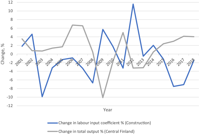
Figure 4. Change in labor input coefficients of construction and total output of the region compared to the previous year (%) in Central Finland 2000–2018.

Production in the region of North Ostrobothnia reduced in 2009 and between 2013 and 2015. In the construction industry in North Ostrobothnia, similar behavior can be observed as in Central Finland (Figure 5). Labor input coefficients and changes in total output vary over the period, but a negative correlation can be seen between them. Changes in the regions can be expected to be larger than on a national level. In addition, variations may be more apparent in percentages than in absolute figures.

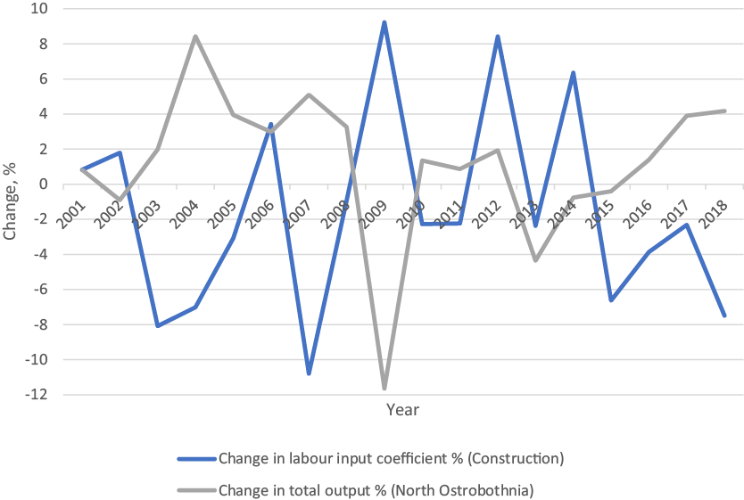
Figure 5. Change in labor input coefficients of construction and total output of the region compared to the previous year (%) in North Ostrobothnia 2000–2018.

Figure 6 shows changes in labor input coefficients and total output in the whole economy in Finland between 2000 and 2018. During the economic boom in the early 2000s, labor input coefficients in construction in Finland declined for several years in a row. As a result of the 2009 recession, labor input coefficients rose, reflecting a fall in labor productivity. The fall in labor productivity may also be due to the implementation of more labor-intensive projects. If raw material prices fall and this lowers the “price” of output, less output is produced for the same amount of labor. At the level of the economy, the variation in labor input coefficients has been smaller than at the regional level in Central Finland or Northern Ostrobothnia.

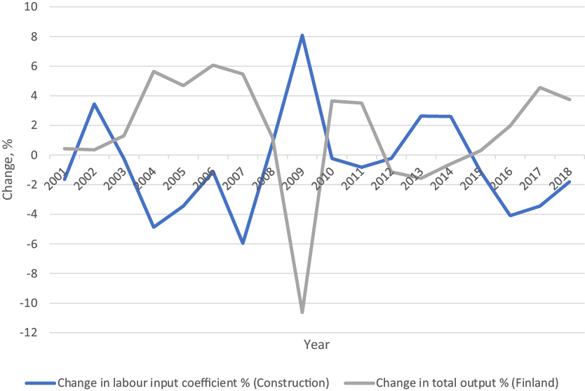
Figure 6. Change in labor input coefficients of construction and total output of the regions compared to the previous year (%) in Finland 2000–2018.

Figure 7 shows the relationship between labor input coefficients and changes in total output for the whole country, Central Finland, and North Ostrobothnia. The correlation is negative in all regions, i.e., labor input coefficients have fallen when the economy has grown and vice versa. The association between labor input coefficients and changes in output is strongest at the level of whole economy in Finland (explanation level R² = 0.72). In Central Finland and North Ostrobothnia, the negative association between these factors is weaker (R² = 0.26−0.33).

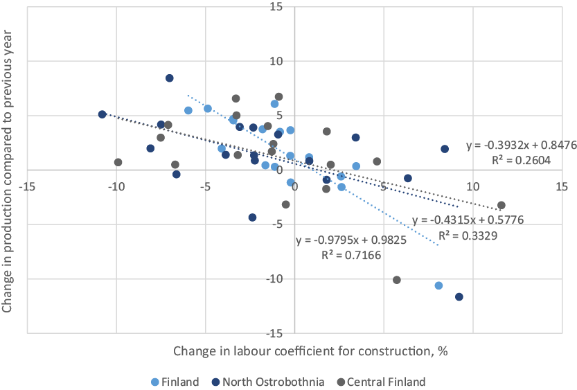
Figure 7. Year-on-year change in construction labor input coefficients and total output (%) in Central Finland, North Ostrobothnia, and Finland 2000–2018.

There is considerable variation in labor input coefficients between years. Economic cycles explain only part of the variation. At the regional level, a significant part of the variation is not explained by the economic cycle. Although it is often difficult to predict future coefficients, historical data and expert opinion can be used to anticipate these changes. Technical progress will continue to improve labor productivity in the future, which is why labor input coefficients can be expected to fall. As labor input coefficients fall, an ever-smaller share of the transport infrastructure construction budget is spent on labor costs. Therefore, the relative employment effects of projects can also be expected to decline in the long term.

Similar observations have been made in Sweden, where the magnitude of the employment effects of road investments during construction has been found to depend on the labor capacity of the construction sector (Trafikanalys, 2012a; Trafikverket, 2015; 2017). Public investment in infrastructure during a boom will crowd out or postpone other public and private investments. At full employment, the labor input required to implement a road investment is completely taken out of alternative use, i.e., the road project crowds out other construction. The use of foreign labor reduces the crowding out effect but, at the same time, it also reduces the effects channeled through changes in domestic consumption demand. However, according to Buchheim and Watzinger (2017), the impact of transport infrastructure projects on other sectors is felt more slowly in the economy than investment in buildings.

There is a clear difference between small investments in repair and maintenance and large investments in infrastructure in terms of counterbalancing the cycles (Trafikanalys, 2012b). On average, low-cost projects are more likely to employ the local businesses and manpower on which they are intended to have an employment impact. In large infrastructure projects, contractors are more often large national companies that subcontract from local companies and employ less local labor on average.

Discussion

Based on the results, we can assert that before choosing an evaluation method (labor input coefficients, input–output model, or computable general equilibrium model), it is essential to define the perspective to be considered and to determine the questions that modeling is intended to answer. Gross employment effects can be estimated with all evaluated assessment methods; however, utilizing the CGE model or labor input coefficients requires multiple modeling iterations or further refinement of results. The CGE model does not directly yield gross effects, as it focuses on economic equilibrium and net employment impacts. Consequently, gross effects necessitate a separate analysis of the model’s intermediate results and require external assumptions from the user, making the CGE model less user-friendly for evaluation purposes. In the three assessed case studies, it was also not feasible to estimate gross effects with the CGE model with a reasonable workload. On the other hand, labor input coefficients are not suitable for estimating employment impacts arising from consumption demand, as they do not reveal the wages generated within the value chain of construction and the resulting consumption demand. The evaluated case projects demonstrated that induced employment impacts were 56% to 75% of direct effects; thus, these can be added to the gross effects using a separate coefficient, which can be derived from other studies if necessary.

The conducted case studies revealed that all evaluation models tend to overestimate direct employment impacts with variations depending on the case and evaluation method ranging from 5% to 50%. Actual direct employment impacts were closest to the results estimated by the IO model in every case, varying between 5% and 21% of the actual direct impacts. When assessed using labor input coefficients, the direct employment impacts were greater than those estimated by the IO model. Conversely, the indirect employment effects were smaller in all evaluation cases. The sum of direct and indirect employment impacts between the labor input coefficients and the IO model varied by 1% to 10% across all evaluation cases.

Examining the realized development of labor input coefficients in the construction sector in Finland in the 2000s, it was observed that the labor input coefficient fluctuated annually across all evaluation regions, with variations from the previous year, between −10.8% and +11.6%. Based on this and the accuracy of different models on ex-ante evaluations, it is crucial to assess the magnitude of the employment impacts generated by transportation infrastructure projects during construction rather than to focus on exact numerical values. Therefore, it is important to choose the most suitable evaluation method based on the need for knowledge to save resources and allocate available planning resources productively rather than trying to model exact employment effects with different models when we know there is some uncertainty.

In principle, if the focus of the study is construction of transport infrastructure and what happens in its production chain, the use of labor input coefficients or IO model is justified and more straightforward than the use of the CGE model. In this case, the modeling results are gross employment effects, i.e., they do not consider the crowding-out effect of the project, but rather the labor demand generated by the projects for the construction itself and other sectors in the value chains. If the overall results are sufficient and there are limited resources available for evaluation, the use of labor input coefficients is justified. If the results are to be examined by industry, the IO model provides additional information, as the results can usually be broken down to the 30–180 industries and induced employment impacts are included in the analysis. In addition, if regional allocations and their structural characteristics are of interest, it is justified to use the MRIO model, where modeling is done at regional levels.

If the research questions are related to the labor markets and, in particular, to the net employment effects, the CGE model provides more answers than labor input coefficients or IO models. The employment effects obtained from input labor coefficients and IO models are gross employment effects and can be further refined to net employment effects by estimating based on assumptions of the kind of labor; e.g., existing labor, unemployed labor, new labor/students, and foreign labor will cover the demand for labor. The assessment can use separate information on the business cycle and regional and national labor markets, using scenario techniques and expert judgment. However, these are based on separate estimates, where resource constraints and the allocation of displacement effects to different regions are not the result of modeling but a given input. The advantage of the CGE model is its ability to take account of resource constraints, allowing the model to estimate the crowding-out effects of projects on other sectors and regions, subject to predefined parameters and constraints.

However, using the CGE model to estimate net employment effects requires an estimate of the labor reserve before modeling, and whether the labor market in the construction of transport infrastructure project area is regional or national, or something in between, related to construction activities and their servicing. In the case projects, the net employment effects depend on the choice of labor market analysis between regional and national analysis. If the labor market is assumed to be regional, the net employment effect is 1.2−1.6 times higher than the direct gross employment effect and 0.7 to 2.0 times higher than realized actual direct employment impacts. If the labor market is assumed to be national, the project will displace labor from other regions and sectors and the net effect will be even slightly negative. In both cases where actual direct employment impacts were known, net employment impacts with national labor market assumptions were 0.4 to 0.5 times negative from the realized actual direct employment impacts.

Traditionally, construction of transport infrastructure has been thought of as a good cyclical policy tool. However, this study concludes that this is not always the case, and the net effect can also be negative even if the gross impact on employment is large. The assessed case study shows that, in a national labor market context, the net employment effects of transport infrastructure investments during construction are small or even negative, unless there is a massive free workforce on the market. This is because the net employment effects depend mainly on the labor reserve, i.e., whether the project has the necessary labor available. If there is a labor reserve, then the increase in investment volume will reduce unemployment and generate a net increase in employment during the construction period. If the skilled labor force is fully employed, the labor force of the new transport infrastructure project is excluded from the labor force of other regions and industries, i.e., the project displaces other productive uses of labor. Therefore, the net effect on employment can be negative if the labor input of the investment displaced by the project under assessment is greater than the labor input of the project itself.

Also, the medium-term economic projections assume that, over a 4-year horizon, labor supply will settle into an equilibrium growth path and that significant cyclical changes will always come unexpectedly. Therefore, there is no justification for examining transport infrastructure investment as a cyclical policy tool. Additionally, obtaining more accurate information on net employment effects—that cannot be obtained by commonly used methods—is not necessary for policymaking, as transport infrastructure should be built because of the need for better connections, not because of an employment policy.

Based on the results of this study, a theoretical and methodological framework was developed for choosing the most suitable evaluation method for assessing the employment effects of transport infrastructure investments during construction. The evaluation framework outlines eight steps through which the construction of transport infrastructure progresses in the economy, simultaneously generating employment effects as well as four more steps to be considered when evaluating net employment impacts. Additionally, the framework specifies which assessment methods can be used to evaluate which impacts. The evaluation framework does not consider possibilities of multiple modeling iterations or further refinement of evaluation results because this would significantly reduce the usability of the models and the comparability of the results (Figure 8).

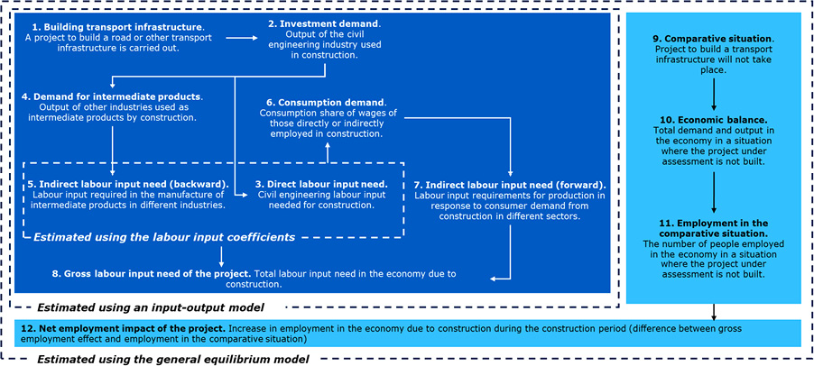
Figure 8. A conceptual evaluation framework for assessing the employment effects of transport infrastructure projects during construction.

The assessment of employment impacts during construction begins with the construction project itself (1), which is the primary activity generating change in the evaluations. The construction project creates investment demand for the construction sector (2), which also requires labor (3). Additionally, various raw materials, intermediate products, and services are required to facilitate the construction process (4). This, in turn, demands labor across multiple industries (5). As a result of the original construction project, both direct (3) and indirect (5) labor demands are generated, which can be estimated using labor input coefficients derived from national accounts.

The investment demand leads to the payment of wage compensations for the work performed, which generates new consumption demand (6), as a significant portion of the wages paid circulates back into the economy through employee consumption. Consumption demand is directed toward various products and services, which again require different raw materials, intermediate products, and labor (7). The employment effects resulting from consumption encompass both direct and indirect employment impacts. By summing the labor demands generated through the various channels (3, 5, and 7), the total gross employment effect of the construction project can be estimated (8). Total gross employment effect can be assessed using the IO model, which describes the interdependencies between industries and the allocation of household consumption across various goods to the industries.

To evaluate net employment effects, a comparative scenario without the project in question is required (9), typically defined as Business-As-Usual (BAU) scenario or the expected trajectory of economic development with existing policy measures (WEM). When assessing net employment effects using the CGE model, the equilibrium state of the economy in the comparative scenario (10) is analyzed to determine the employment in the comparative situation and sectoral distribution (11), reflecting the anticipated economic development without the evaluated construction project. By subtracting the employment in the comparative scenario (11) from the gross employment effects of the construction project (8), the net employment effect of the project becomes evident (12). The suitability and usability of the methods, as well as the need for prior information, have been summarized in Table 7, rated on Likert scale of poor–moderate–good.

**Table 7. Suitability and usability of the methods, and the need for prior information, rated on a Likert scale of poor–moderate–good.**
	Labor input coefficients	Input–output model	Computable general equilibrium model
Suitable to evaluate overall gross employment effects	Moderate	Good	Poor
Suitable to evaluate overall net employment effects	Poor	Poor	Good
Suitable to evaluate employment effects by industry	Poor	Good	Good
Suitable to evaluate employment effects by regions	Poor	Good	Good
Ease of use and comprehension	Good	Moderate	Poor
No need for prior data	Good	Moderate	Poor

Net employment effects are examined at both the industry and regional levels, allowing for individual job movements between different companies and sectors, which may be positive for some and negative for others, even if this is not reflected in the overall impacts. The CGE model is the only one among the evaluated models that allows for the estimation of net employment effects through modeling, rather than relying on scenarios defined outside the models, which always involve uncertainties and challenges in presenting them consistently.

There are no restrictions on the use of the evaluation framework based on the size or type of projects; however, the key limitations relate to the availability of data on regional and national labor markets and labor mobility. As observed in the case projects, the CGE model is quite sensitive to labor market assumptions, meaning that incorrect labor market assumptions can significantly affect net employment impacts. If sufficient information on labor markets is not available, it may be prudent to focus solely on determining the magnitude of gross employment effects, as future labor demand is also crucial information when planning various projects.

Conclusions

The objective of this research was to outline a methodological framework for selecting suitable ex-ante evaluation methods to assess the employment impacts of transport infrastructure investments during construction. Based on literature and real case projects, this study developed a framework that helps to define the right evaluation methods based on the needed knowledge and perspectives. Each modeling approach presented in the framework has its own advantages and limitations, with decision-making situations and perspectives determining which is the preferred way to provide additional information to support decision-making.

The amount of labor required for construction of transport infrastructure projects can be estimated with sufficient accuracy using the input–output statistics’ labor input coefficients. However, it is useful to consider the changing environment by including a range for the labor input factor in the assessment based on time series. The investment in on-site labor and intermediate manufacturing is a feature of the project, alongside the cost estimate. The presentation of labor needs alongside the cost estimate would be potentially useful in two ways. First, it would put the gross employment impact of the project during construction in its proper context, i.e., as a cost-dependent labor input. This would avoid confusing the effort required with the benefits that will be accrued because of the project. Second, an estimate of labor needs can be a useful input for programming the timing of transport infrastructure projects in different regions, if at the same time, estimates of employment in infrastructure engineering and related industries in different regions are available.

It is recommended that the assessment of labor needs is added to the project appraisal of transport infrastructure investments as a more detailed analysis of the cost estimate, based on statistical data. It offers opportunities to examine the demand for labor in the future, for example, in terms of skills and resources.

If the need for knowledge is related to net employment effects, a computable general equilibrium model is the most suitable method, but it requires an assessment of the labor market situation and labor supply before modeling. The net employment effects can also be evaluated based on coefficients or a static input–output model, but additional information is needed to further refine the modeling results into net employment effects. Even then, the impacts are based on scenario techniques and assumptions about the channels through which employment demand will be met.

References

Adema, Y. and Pozzi, L. 2015. Business cycle fluctuations and household saving in OECD countries: A panel data analysis. European economic review, 79, pp. 214-233. https://doi.org/10.1016/j.euroecorev.2015.07.014
Alho K. 2002. The Equilibrium Rate of Unemployment and Policies to lower It: The Case of Finland. No 839, Discussion Papers from The Research Institute of the Finnish Economy. https://EconPapers.repec.org/RePEc:rif:dpaper:839
Alloza, M. and Sanz, C. 2021. Jobs Multipliers: Evidence from a Large Fiscal Stimulus in Spain. The Scandinavian journal of economics, 123(3), pp. 751-779. https://doi.org/10.1111/sjoe.12428
Anagnostou, A. and Gajewski, P. 2021. Multi-regional input-output tables for macroeconomic simulations in Poland’s regions. Economies, 9(4), pp. 1-19. https://doi.org/10.3390/economies9040143
Buchheim, L. and Watzinger, M. 2017. The Employment Effects of Countercyclical Infrastructure Investments. Social Science Research Network. https://doi.org/10.2139/ssrn.2928165
Dimitriou, D. and Sartzetaki, M. 2022. Assessment of Socioeconomic Impact Diversification from Transport Infrastructure Projects: The Case of a New Regional Airport. Transportation research record, 2676(4), pp. 732-745. https://doi.org/10.1177/03611981211064999
Dixon, P and Jorgenson, D. 2012. Handbook of Computable General Equilibrium Modeling. 1st ed Edition, Volume 1A. North Holland. https://doi.org/10.1016/B978-0-444-59568-3.00062-6
ELY Centre. 2015. Pyhäjoen ydinvoimalan edellyttämät tieinvestoinnit: Hankearviointi [Road investments required for the Pyhäjoki nuclear power plant: Project evaluation]. North Ostrobothnia Centre for Economic Development, Transport and the Environment. Reports 37/2015. https://urn.fi/URN:ISBN:978-952-314-253-4
Ernst, C. and Marianela S. 2015. The role of construction as an employment provider: a world-wide input-output analysis. ILO Working Papers 994891843402676, International Labour Organization. https://econpapers.repec.org/paper/iloilowps/994891843402676.htm
European Commission (2014). Guide to Cost-Benefit Analysis of Investment Projects, Economic appraisal tool for Cohesion Policy 2014–2020. https://doi.org/10.2776/97516
Finnish Transport Agency. 2017. Perusväylänpito ja liikenneväylien korjausvelkaohjelma 2016–2018 [Basic road maintenance and road repair deck programme 2016–2018]. Interim report 6/2017 Finnish Transport Agency
Finnish Transport Infrastructure Agency. 2017. Äänekosken biotuotetehtaan liikenneyhteydet [Transport links to the Äänekoski bioproduct plant]. Tampere-Jyväskylä-Äänekoski railway project. The final results of the project. 15.8.2017. Finnish Transport Infrastructure Agency. VR Track Oy.
Finnish Transport Infrastructure Agency. 2021. VT 8 Pyhäjoki - Liminka. [Online] Available at https://vayla.fi/vt8pyhajoki. [Accessed 8 November 2021].
Garin, A. 2019. Putting America to work, where? Evidence on the effectiveness of infrastructure construction as a locally targeted employment policy. Journal of urban economics, 111, pp. 108-131. https://doi.org/10.1016/j.jue.2019.04.003
Hokkanen, J., Savikko, H., Känkänen, R., Sirkiä, A., Virtanen, Y., Katajajuuri, J-M. and Sinkko, T. 2017. 27. A Regional Resource Flow Model for promoting a circular economy at the regional level. In the book: Ludwig, C., Matasci, C. (Eds.) World Resource Forum. Boosting resource productivity by Adopting the Circular Economy. pp 205 – 209. ISBN 978-3-9521409-7-0. available: https://www.wrforum.org/wp-content/uploads/2017/10/Ludwig_2017_WRF_book_FINAL.pdf
Honkatukia, J. 2009. VATTAGE - A dynamic, applied general equilibrium model of the Finnish economy. Research Reports 150, VATT Institute for Economic Research. available: https://urn.fi/URN:ISBN:978-951-561-875-7
Honkatukia, J. 2013. The VATTAGE Regional Model VERM - A Dynamic, Regional, Applied General Equilibrium Model of the Finnish Economy. VATT Research Reports No. 171, https://doi.org/10.2139/ssrn.2284665
Honkatukia J., Lehtomaa, J., Alimov, N., Huovari, J. and Ruuskanen, O-P. 2019. Alueellisen taloustiedon tietokanta [Regional economic database]. Publications of the Government´s analysis, assessment and research activities 41:2019. available: http://urn.fi/URN:ISBN:978-952-287-753-6
Langston, C. and Crowley, C. 2021. Evaluation of transportation infrastructure: A case study of gold coast light rail stage 1 and 2. Construction economics and building, 21(4), pp. 1-20. https://doi.org/10.5130/AJCEB.v21i4.7738
Laird, J. J. and Venables, A. J. 2017. Transport investment and economic performance: A framework for project appraisal. Transport policy, 56, pp. 1-11. https://doi.org/10.1016/j.tranpol.2017.02.006
Leontief, W. and Strout, A. 1963. Multiregional Input-Output Analysis. In: Barna, T. (ed.) Structural Interdependence and Economic Development. Palgrave Macmillan, London. https://doi.org/10.1007/978-1-349-81634-7_8
Lieuw-Kie-Song, M., Abebe, H., Sempundu, T. and Bynens, E. 2019. Employment impact assessments analysis of the employment effects of infrastructure investment in Rwanda using multiplier analysis of construction subsectors. IDEAS Working Paper Series from RePEc.
Markaki, M. and Belegri-Roboli, A. 2010. Employment determinants in an input-output framework: structural decomposition analysis and production technology. Bulletin of political economy. 4. pp. 145-156.
McMorrow K.C. and Roeger, R. 2000. Time-Varying Nairu/Nawru. Estimates for the EU’s Member States. Economic papers 145, ECFIN. https://aei.pitt.edu/34753/1/EP145.pdf
Miller, R. E. and Blair, P. D. 2009. Input-Output Analysis Foundations and Extensions. 2nd Edition. Cambridge. Cambridge University Press. 784 p. https://doi.org/10.1017/CBO9780511626982
Moszoro, M. 2021. The Direct Employment Impact of Public Investment. IMF Working Paper Fiscal Affairs Department. Working Paper No. 2021/131. https://doi.org/10.5089/9781513573793.001
OSF 2021a. Official Statistics of Finland (OSF): Input-output [e-publication]. ISSN=1799-201X. Helsinki: Statistics Finland [referred: 18.10.2021]. available: http://www.stat.fi/til/pt/index_en.html
OSF 2021b. Official Statistics of Finland (OSF): Regional accounts [e-publication] Helsinki: Statistics Finland [accessed: 16.11.2021]. available: http://www.stat.fi/til/altp/meta.html
Pienaar, W. J. 2024. Impact of rural road provision on employment. South African journal of industrial engineering, 35(1), pp. 31-40. https://doi.org/10.7166/35-1-2912
Purwanto, A., Heyndrickx, C., Kiel, J., Betancor. O., Socorro M. P, Hernandez, A., Eugenio-Martin, J.L, Pawlowska, B., Przemyslaw, B. and Fiedler, R. 2017. Impact of Transport Infrastructure on International Competitiveness of Europe. Transportation Research Procedia (Online), 25. pp. 2877–2888. https://doi.org/10.1016/j.trpro.2017.05.273
de Rus, G., Socorro, M. P., Valido, J. & Campos, J. 2022. Cost-benefit analysis of transport projects: Theoretical framework and practical rules. Transport policy, 123, pp. 25-39. https://doi.org/10.1016/j.tranpol.2022.04.008
Savikko, H. 2014. Alueelliset resurssivirrat Jyväskylän seudulla [Regional resource flows in the Jyväskylä region]. Master’s thesis, Tampere University of Technology, Department of Industrial management.
Savikko, H., Hokkanen, J., Metsäranta, H., Sirkiä, A., Ilomäki, R. 2021. Polttoaineen hinnannousun yritysvaikutukset [The effects on businesses of the rise in fuel price]. Government Reports of Prime Minister’s Office of Finland, 2021:5. available: http://urn.fi/URN:NBN:fi-fe2021101851335
Teo, P., Gajanayake, A., Jayasuriya, S., Izaddoost, A., Perera, T., Naderpajouh, N. and Wong, P. S. 2022. Application of a bottom-up approach to estimate economic impacts of building maintenance projects: Cladding rectification program in Australia. Engineering, construction, and architectural management, 29(1), pp. 333-353. https://doi.org/10.1108/ECAM-10-2020-0802
Trafikanalys (2012a). Anläggningsbranschen – utveckling, marknadsstruktur och kon-junkturkänslighet [The Construction Industry – Development, Market Structure, and Sensitivity to Economic Cycles]. Trafikanalys PM 2012:1.
Trafikanalys (2012b). Infrastrukturåtgärder som stabiliseringspolitiskt instrument – redovisning av ett regeringsuppdrag [Infrastructure Measures as a Stabilization Policy Instrument – Reporting on a Government Assignment]. Trafikanalys Rapport 2012:1.
Trafikverket (2015). Krav på sysselsättning i upphandlingar, Redovisning av ett regeringsuppdrag [Requirements for Employment in Procurement, Reporting on a Government Assignment.]. Trafikverket. TRV 2015/57193.
Trafikverket (2017). Teoretiska utgångspunkter för koppling mellan åtgärder i nationell plan och sysselsättning [Theoretical Foundations for the Connection Between Measures in the National Plan and Employment]. PM till Nationell plan för transportsystemet 2018-2029. Trafik-verket. TRV 2017/32405.
Wang, B. 2015. Estimating economic impacts of transport investments using TREDIS: a case study on a National Highway Upgrade Program. Paper Presented at Australasian Transport Research Forum 2015, 30 September – 2 October 2015, Sydney, Australia, available at: https://australasiantransportresearchforum.org.au/wp-content/uploads/2022/03/ATRF2015_Resubmission_180.pdf (accessed 4 April 2025).
Wilson, D. J. 2012. Fiscal Spending Jobs Multipliers: Evidence from the 2009 American Recovery and Reinvestment Act. American economic journal. Economic policy, 4(3), pp. 251-282. https://doi.org/10.1257/pol.4.3.251
World Bank (2021). Jobs and Distributive Effects of Infrastructure Investment. © World Bank. Available at: https://documents1.worldbank.org/curated/en/721891623745711077/pdf/Jobs-and-Distributive-Effects-of-Infrastructure-Investment-The-Case-of-Argentina.pdf