Construction Economics and Building

Vol. 25, No. 2
July 2025

RESEARCH ARTICLE

Enlightening the Critical Factors Affecting the Solvency of Indian Construction Industry: An Empirical Analysis Using Multivariate Discriminant Analysis and Logistic Regression

Rakesh Kumar Sharma^1,*, Neba Bhalla²

¹ Department of Humanities and Social Sciences, Thapar Institute of Engineering and Technology (Deemed to be University), Patiala 147004 Punjab

² School of Business, UPES (University of Petroleum and Energy Studies), Kandoli, Dehradun, Uttarakhand

Corresponding author: Rakesh Kumar Sharma, Department of Humanities and Social Sciences, Thapar Institute of Engineering and Technology (Deemed to be University), Patiala 147004 Punjab, rakesh.kumar@thapar.edu

DOI: https://doi.org/10.5130/AJCEB.v25i2.8752

Article History: Received 03/08/2023; Revised 02/12/2023; Accepted 01/01/2024; Published 08/08/2025

Citation: Sharma, R., Bhalla, N. 2025. Enlightening the Critical Factors Affecting the Solvency of Indian Construction Industry: An Empirical Analysis Using Multivariate Discriminant Analysis and Logistic Regression. Construction Economics and Building, 25:2, 276–302. https://doi.org/10.5130/AJCEB.v25i2.8752

Abstract

The present research work aimed to examine the vital factors that affect the solvency of the Indian construction sector. The two different parameters of solvency, namely, debt to total assets (DTA) and cash flow to total liabilities (CFTL), were used in the present study. These two solvency indicators were categorized using zero and one numerical values. One indicates financially sound companies, and zero indicates weak companies with poor solvency ratios. The different financial ratios, namely, profitability, liquidity, leverages, and turnovers, were used as predictors or explanatory variables of insolvency of Indian construction companies. The study employs multivariate discriminant analysis (MDA) and binary logistic regression to predict the factors accountable for the insolvency of the Indian construction sector. The empirical findings of MDA and logistic regression show significant discrimination in the solvency position of construction companies according to their different financial performance parameters, namely, profitability, liquidity, and leverage. The empirical findings suggest that in the first case, the critical indicators predicting solvency are turnover, liquidity, and leverage ratios. In the second measure of solvency (CFTL), profitability significantly discriminates solvency of companies. Overall, the findings of MDA and logistic regression are consistent with each other. The outcomes of the study will be helpful to policymakers’ different stakeholders.

Keywords

Solvency Ratios; Profitability Ratios; Activity Ratios; Leverage; Multivariate Discriminant Analysis

JEL classification

G33, G32, G17, G01, C3

Introduction

The construction industry in India has become the second-largest employer and foreign direct investment (FDI) recipient in 2020–2021 and the third-largest market globally. India’s construction industry attracted nearly 5 billion USD of investment in 2020, leading to predicted average growth of 7% every year until 2025 (Rani, 2021). The sector that contributes directly to the country’s overall development is the construction sector. According to Statista Research Department, in July 2020, the Indian construction industry was worth over 1.3 trillion Indian rupees (Statista, 2024).

The nature of the construction sector is a project-based industry under which different parties like contractors, clients, and consultants have to work collectively to complete a project. The failure or success of the construction sector notably affects the other sectors associated with them. The construction sector’s performance can affect the national budget, so there is a need to develop proficient planning in executing the projects. Hence, the project manager should look for efficient tools and techniques. In India, real estate is forecast to stretch out to 650 billion USD, exhibiting 13% of India’s gross domestic product (GDP) by 2025. The government of India has allowed FDI of 100% for townships and settlements. India’s real estate attracted over 6.06 billion USD in investment in India. The role of the construction sector is significant in the Indian economy. From the financial year 2010 to the financial year 2015, the growth rate of this sector was up at 2.95%, and the growth rate of the construction sector across India was evaluated to be 5.65% from the financial year 2015 to 2022 (Statista, 2024).

However, after the global financial crisis, the Asian financial crisis in 2014, the introduction of demonetization and Goods and Services Tax in 2017, and the coronavirus disease 2019 (COVID-19) pandemic in 2020 have been worrying for the Indian economy. Subsequently, India’s GDP has declined to 10.29% from 8.0%.

Therefore, there is an urgent requirement that the government and related stakeholders examine the critical factors that influence the financial state of Indian construction companies. There is a need to conduct a detailed analysis of the essential factors affecting the solvency of the Indian construction industry. Muresan and Wolitzer (2004) described financial ratio analysis as being helpful over the years to give a holistic stance of a company’s financial position at any point or period.

Financial ratios are significant numerical values extracted from accounting statements to obtain relevant information about a company. Traditionally, financial ratios are categorized mainly into current, solvency, profitability, and activity ratios (Paramasivan and Subramanian, 2008).

To check whether a company has sufficient cash flow or not to manage its debt liabilities that are due, solvency ratios play a significant role. Another name for the solvency ratio is the leverage ratio. A company with a low solvency ratio signifies more risk of fulfilling its debt obligation and vice versa. In the presence of a large number of companies in a particular sector, it is impractical to examine all the ratios every time to determine an industry’s financial state. Moreover, no one ratio describes the complete information about the company, whereas the random combination of ratios may lead to redundancy in the report. Thus, there is a need to find out the significant ratios of the Indian construction companies and consequently discover the critical factors that influence the financial health of the Indian construction companies.

Literature review

Financial ratio analysis is one of the most important and common ways to examine the economic progress and growth of companies in the construction industry in different countries (Kim and Zhang 2014). Balatbat, Siew, and Carmichael (2020), and Rajala, et al. (2022) all included financial ratios in their research. Each researcher can apply specific financial ratios and factors that signify the research objectives they aim to achieve for a certain number of years. Profitability and liquidity ratios such as the net profit margin and current ratio are used in various studies (Wang and Lee, 2008; Niemann, Schmidt, and Neukirchen, 2008; Sansusi, et al., 2017).

Moyer (1990) explained financial ratios for three purposes. The first is to measure the firm’s feasibility and identify the weaknesses and strengths of the firm. Second, in planning to achieve the company’s goals, financial ratios play an essential role, and third is to ensure the company objectives are well suited to its resources. With the help of financial ratios, a market analyst can compare a firm’s financial condition with that of other firms over time. Vibhakar, et al. (2023) also investigated that financial ratios compare a company’s financial performance over time with itself and with that of other firms within the same industry.

Pamulu, Kajewski and Betts (2007) examined the financial ratios of Indonesian firms in the construction sector. The results reveal that Indonesian companies are financially sound, whereas profits and returns produced from construction works are quite satisfactory. Suber (2011) analyzed the financial health of Malaysian construction firms with the help of financial ratio analysis to examine the performance and compare the company’s performance with that of other companies and industries; the research found that a weak liquidity ratio, cash, and capital would be inadequate to finance construction projects. It is a vital sign that companies are undercapitalized and can face financial problems in the future.

The most common criteria employed to determine the financial performance of construction firms are return on investment, turnover, profit, etc. A construction project is deemed successful if it is done within specifications and without cost overruns (Tripathi and Jha, 2018; Dong, et al., 2022). However, construction firms having an excellent track record of successful projects do not always guarantee the success of the construction organization. Despite its projects’ success, construction organizations can even fail or become insolvent due to the high risk in the business (Jha, 2015). Success can be expressed as the point at which the expectations and objectives of a company are fulfilled. In contrast, the failure of a company is caused by its inefficacy to complete its commitment when it is due (Arslan and Kivrak, 2008).

De Franco, Kothari and Verdi (2011) investigated to recognize the critical financial points. The results show factor analysis on 44 financial ratios to reduce them to 25 important variables, categorized into eight sets for the Indian cement industry. They analyzed eight significant factors: short-term liquidity, return on investment and profitability, long-term solvency, cash position, asset and material management, dividend policy, capital structure, and working capital productivity. They applied multiple regression analysis between the factor scores and constituent variables to exclude the statistically insignificant variables.

Javalagi and Bhushi (2007) also analyzed the financial performance of the Indian industry by implementing factor analysis to recognize the six financial factors, i.e., cash to current liabilities, working capital, retained profits, financial leverage, inventory, and profitability. Chan and Au (2009) examined the financial health of different parties or contractors during the Asian economic turbulence. They tried to assess and monitor financial well-being by applying the accounting ratios with the help of Altman’s distress models. Tsolas (2011) investigated the achievement of construction companies registered in the Athens Exchange, evaluated the financial soundness in terms of effectiveness and profitability, and outlined a new structure that united ratio analysis and data envelopment analysis (DEA).

Chen (2011) analyzed macroeconomic and financial points to predict sales of construction companies. In contrast, Kehinde and Mosaku (2006) used ratio analysis to analyze medium-sized construction companies’ assets in Nigeria. Niemann, Schmidt and Neukirchen (2008) applied financial ratios for rating prediction models for multinational corporations.

Horta, et al. (2013) came up with a quantitative approach to examine construction firms’ financial strength and discover the factors that promote innovation and performance improvements using data envelopment analysis and regression analysis. Ramalho and da Silva (2013) analyzed the fraction regression model, features of Tobit models, and econometric assumptions to give a conceptual basis for their application in the regression study of various leverage ratios.

Investors use the solvency ratios and liquidity ratios as tools to make their investment decisions. Solvency ratios assess the firm’s ability to meet its financial obligation when it is outstanding. Most empirical studies evidence the relationship between liquidity, activity, profitability, and leverage with the solvency of a firm.

The following literature provides a deeper insight into the relationship of all the variables that impact the solvency of a firm.

Relationship with profitability

Good performance and financial position are needed for business entities to operate in the future (Jeon, Amekudzi, and Guensler, 2010). Profitability and solvency are often exercised as a benchmark to measure financial position and performance (Kiyosaki and Lechter, 2003). Profitability analysis is an essential instrument for decision-making and management planning, as it generates value for the firm (Penman, 2007). Vieria (2011) stated that the evaluation of profitability is generally done with the help of return on equity and return on assets. Khalid and Rehman (2014) examined a negative relationship between profitability inconsistency and solvency. Less profitable firms delay the payment of routine expenses of the company. A study conducted in Ghana by Addae, Nyarko-Bassi, and Hughes (2013) stated a positive relationship between short-term debt and profitability compared to long-term debts.

Moreover, a positive relationship occurs between the solvency levels per the pecking order theory. A profitable firm can survive in any adverse situation and use its retained earnings well (Arvanitis, et al., 2012). Bordeleau and Graham (2010) stated that at some point over, liquidity had reduced the profitability level of firms. Mohanty and Mehrotra (2018) stated a significant relationship between profitability and return on assets (ROA) and not a statistically significant relationship between solvency and return on equity (ROE). Solvency has no impact on profitability, but liquidity negatively impacts it (Dahiyat, Weshah and Al-Dahiyat, 2021).

H1: The different measures of profitability can distinguish between strong solvent and weak solvent Indian construction companies.

Relationship with liquidity

A company’s capacity to fulfill its short-term obligations and manage the cash requirements to operate the business smoothly is measured through liquidity ratios (Hayes, 2019). The liquidity position is a measure to analyze the company’s capacity to discharge its current liabilities with current assets. The company’s liquidity position is considered better if higher (Loncan and Caldeira, 2014). Working capital management is essential, as it directly affects its solvency (Singh and Pandey, 2008). The working capital directly influences the solvency of a firm. Negative working capital leads a firm to bankruptcy (Panigrahi, 2014). The financial structure is directly associated with high profitability, liquidity, and solvency. Here, financial structure is implied by working capital management (Guimaraes and Nossa, 2010). Khalid and Rehman (2014) stated that the higher the quick and current ratio is, the more the company can easily handle the cash troubles. Moorthi, et al. (2012) stated that liquidity plays an essential role in the existence of a business. It affects solvency, i.e., the ability to survive in the long run. Silva (2019) stated that too much liquidity has a negative implication on the solvency of a firm.

Research conducted in Saudi Arabia by Eljelly (2004) analyzed that profitability is assessed by the cash conversion cycle and the current ratio and identified a link between profitability and the solvency of a firm. Carslaw and Mills (1991) stated that cash flow is used to ascertain short-term financial stability. It is an indicator used to measure a firm’s financial risk. Ben, Olubukunola and Uwuigbe (2013) and Ademola, et al. (2020) examined the Nigerian Stock Exchange and stated that the current liquidity ratio is positively related to profitability. It helps to ascertain the solvency position of a firm. A study on the Malaysian manufacturing sector measured liquidity using the working capital and current ratio to total asset ratio. It states that a positive relationship prevails between the profitability and liquidity of a firm (Zainudin, et al., 2017).

H2: Liquidity of selected companies can discriminate them into very healthy and unhealthy Indian construction companies.

Relationship with activity ratios

Activity ratios are the performance measuring tools of a firm and express the organization’s operational capabilities. A higher ratio means better utilization of the resources. Financial challenges have been a significant worry since the financial crisis of 2008. Activity ratios help in evaluating financial efficiency and performance. A study showed the direct relationship of activity and profitability ratios with the solvency of the firms (Rawat, et al., 2022). The Serbian enterprise study uses cash flow investing margin and cash flow operating margin as liquidity yardsticks. The cash flow operating margin shows a negative impact, and the cash flow investing margin has a positive repercussion. The indicator used for the cash flow investing margin is the cash invested in a firm’s fixed assets . Drobetz, et al. (2013) stated that organizations having a higher ratio of fixed to total assets bear low financial distress. There is less chance of them suffering higher losses at times of insolvency or bankruptcy. The turnover ratios analyze the enterprise’s sales ability; the higher the turnover ratio, the higher the benefit for the firm (Xia, et al., 2023). The analysis of activity ratios helps to improve operational efficiency (Zhu, et al., 2019).

H3: The different measures of activity ratios can distinguish between strong solvent and weak solvent Indian construction companies.

Relationship with leverage ratios

A company’s survival depends on its capital structure and not just its earning potential. Leverage ratios tell the proportion of debt used in the firm’s capital structure. Pandey and Bhat (1990) and Bhat, Chanda and Bhat (2023) examined the financial leverage of Indian manufacturing industries. They employed various factors such as firm dividend payout ratio, income variability, size, and growth. Their studies deduced that a firm’s size is not related to financial leverage. However, a firm is riskier in terms of solvency when it is likely to employ more percentage of debt in comparison with financial leverage and earnings before interest and tax (EBIT). Abey and Velumurugan (2019) stated that capital structure determines the company’s survival in the future and long-term solvency. Their study used the variables of return on investment, size of the company, and asset structure to determine the financial leverage of the Indian automobile industry. Yeo (2016) stated that leverage is closely and directly related to solvency. A firm should only accelerate the intake of debts when it is affirmative to get higher returns.

Moreover, the study identified that variables like profitability and size of the firm also influence the leverage level. Durand (2019) stated that capital positively impacts financial stability in terms of solvency at a low level. However, when the capital increases, the solvency of a firm becomes weaker. The financial leverage ratio helps to measure the financial performance of operations. It is of great value to investors, creditors, and managers in the long run (Andrew, Damitio, and Schmidgall, 2007). The turnover ratios give a comprehensive approach to analyzing the solvency position of the firms (Kajananthan and Velnampy, 2014). A study on manufacturing companies in Nigeria showed that solvency in terms of credit policies, cash conversion, and earnings plays an essential role in corporate profitability (Owolabi and Obida, 2012). In their study, Graham and Leary (2011) stated that firms with lower bond ratings and more debt are more prone to insolvency and financial distress. Bonaccorsi di Patti, et al. (2015) stated the two-fold impact of leverage on firms. First, firms default during economic contractions. Second, leverage increases the sensitivity of the firm.

H4: Leverage ratios of selected companies can separate them into very healthy and unhealthy Indian construction companies.

Research design or research methods

This study was carried out by procuring the different explanatory and dependent variables from Prowess, the Centre for Monitoring Indian Economy (CMIE). The study period was from the last 10 years, from 2011 to 2020. The two different solvency parameters used in the study were cash profit after tax to total liabilities and debt to total assets of Indian construction sector companies.

There cannot be a single reason for insolvency; by keeping this in mind, the study included the different financial ratios as explanatory variables. These ratios deal with profitability, short- and long-term financial position, and managerial efficiency or activity ratios of the Indian construction companies.

At the initial stage, data on a total of 3,947 companies were procured. However, the companies that shut down their business during the study period were excluded from the sample. Similarly, the companies whose complete data set of the last 10 years of different explanatory and dependent variables were not available were also dropped from the sample size. At last, a sample of 148 construction companies was taken. Data of all the variables as mentioned earlier were collected for the time of 2011 to 2020. Multivariate discriminant analysis (MDA) and binary logistic regression are used to predict the solvency of selected Indian construction companies.

The methods adopted to conduct the research are MDA and Binary Logistic Regression as explained in Section 3.1 and 3.2. Furthermore, the variables for each financial ratio selected for evaluating the solvency ratios are specified in section 3.3

Multivariate discriminant analysis (MDA)

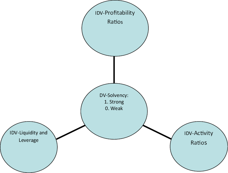
Multivariate discriminant analysis is identical to multiple regression analysis. The only point of distinction is that in the case of MDA, the dependent variable is qualitative, whereas in the case of multiple regressions, this variable is quantitative. In multiple regressions, there is more than one independent variable. There is also more than one independent variable in MDA. There is a single dependent variable in the multiple regressions, whereas the dependent variable is categorical in the case of MDA. In the present paper, the dependent variables were the different categories of the solvency ratio of selected companies. These different solvency indicators were categorized using two numerical values: one and zero (Refer to Figure 1). One indicates that those companies with a sound financial position and overall health are very good; zero reflects that companies having poor solvency ratios are weak companies. The different financial ratios, viz., profitability, liquidity, leverage, and activity, were used as predictors or explanatory variables of the insolvency of Indian construction sector companies.

Figure 1. MDA variables.

Source: Authors’ Compilation

The discriminant equation in the present study is as follows:

Z = β0 + β1 (Profitability) + β2 (Liquidity) + β3 (Leverage) + β4 (Activity) + ε, 1

where Z is the latent categorical variable. Profitability, liquidity, leverage, and activity ratios are the explanatory variables. β0 is the intercept or constant. β1, β2, β3, and β4 are the coefficients to calculate the discriminant score. ε is the error term.

Binary logistic regression (BLR)

Furthermore, binary logistic regression was used in the current study to authenticate MDA results. In the case of binary logistic regression, the dependent variable was the two categories of companies: strong solvent companies and weak solvent companies. These companies were categorized using binary numbers, where one indicates strong solvent and zero weak solvent companies. The study used a forward logistic regression (LR), and the forward LR is similar to stepwise multiple regression. It adds the significant independent variables in each subsequent stage. Forward LR (Xie, et al., 2013) removes explanatory variables that are not significant. The remaining independent variables are the significant independent variables used to calculate the discriminant score. Like multiple regression, binary logistic regression also measures the cause-and-effect relationship among independent and dependent variables by converting the explanatory variables to probability scores, i.e., zero and one. In the logit model, the odds ratio is expressed as the probability of a high impact to a low impact (i.e., no impact) or P(H)/1 − P(H). The model under logit regression is expressed as a linear function of the company’s predictor variables.

$L o g \frac{P (H)}{1 - P (H)} = α_{0} + α_{1} X_{i 1} + \dots \dots . + α_{n} X_{i n}$ (1)

where P(H) is the probability of having a high impact on the ith construction companies: α₀ is an intercept; X₁ − X_n are the latent variables; α₁ − α_n are the coefficients of the nth latent variables. Liao (1994) opined that Equation (1) could be changed into a description of the logistic regression model of event probability.

Calculating P(H) through Equation (1), the expected probability of having a high impact is described as follows:

$P (H) = \frac{1}{[1 + e^{- z}]}$ , $z = α_{0} + α_{1} X_{i 1} + \dots \dots . + α_{n} X_{i n}$

In the above equation, the base of the natural logarithm is “e”.

The present logistic model uses different financial ratios associated with leverage, profitability, liquidity, and turnovers as predictor variables. These ratios are assumed to split the companies into strong solvent and weak solvent companies.

The respective logit equation for business performance (operational performance, cost, and profitability) is as follows:

$P (H) = \frac{1}{[1 + e^{- z}]}$ ,

where

Z = α + β_{1} {(l e v e r a g e)}_{i 1} + β_{2} {(p r o f i t a b i l i t y)}_{i 2} + β_{3} {(l i q u i d i t y)}_{i 3} + β_{4} {(t u r n o v e r r a t i o s)}_{i 4} + ε

Binary logistic regression has been used to predict different financial ratios affecting business solvency. Values zero (for weak solvent companies) and one (for strong solvent companies) are assigned to dependent variables: solvency. The average is calculated based on the measuring scale used for each dependent variable. Accordingly, values zero and one are assigned as shown in Table 3 to measure the impact using logistic regression.

Dependent and independent variables

This section highlights the variables selected as dependent and independent variables for financial ratios to predict the solvency of Indian construction companies as stated in Table 1.

**Table 1. Definition of different independent and dependent variables.**
Ratios		Calculation	References
Profitability ratios	Net profit ratio (NPR)	Net profit/Net sales	Jeon, Amekudzi and Guensler (2010); Kiyosaki and Lechter (2003); Penman (2007); Vieria (2011); Khalid and Rehman (2014); Addae, Nyarkao-Bassi and Hughes (2013); Arvanitis, et al. (2012); Bordeleau and Graham (2010); Mohanty and Mehrotra (2018); Dahiyat, Weshah and Al-Dahiyat (2021)
	Profit before tax ratio (PBTR)	PBT/Net sales
	Profit after tax ratio (PATR)	PAT/Net sales
	Cash profit ratio (CPR)	Profit after tax + Non-cash expenses – Non-cash incomes/Net sales
	Return on assets (ROA)	EBIT/Total assets
	Return on equity (ROE)	PAT − Preference dividend (if any)/Equity shareholders’ funds
	Return on sales or operating profit ratio (ROS)	Operating profit/Net sales
Liquidity ratio	Current ratio	Current assets/Current liabilities	Loncan and Calderia (2014); Singh and Pandey (2008); Panigrahi (2014); Khalid and Rahman (2014); Moorthi, Ramesh and Bhanupriya (2012); Silva (2019); Eljelly (2004); Carslaw and Mills (1991); Ben, Olubukunola and Uwuigbe (2013) and Ademola, et al. (2020);Zainudin, et al., 2017 Guimaraes and Nossa (2010)
Activity ratios	Total asset turnover	Net sales/Total assets	Drobetz, et al. (2013); Zhu, et al. (2019)
	Fixed asset turnover	Net sales/Fixed assets
	Working capital asset turnover	Net sales/Net working capital
	Current asset turnover	Net sales/Current assets
Leverage	Financial leverage	Debt to Equity ratio	Bhat, Chanda and Bhat (2023); Abey and Velumurugan (2019); Yeo (2016); Durand (2019); Andrew and Schmidgall (1993); Kajananthan and Velnampy (2014); Owolabi and Obida (2012); Patti, et al. (2015)
		Earnings before interest and tax/Earning before tax
		Total debt to Sales
Solvency ratios	Debt to total liabilities (DTL)	Debts/Total liabilities	Cook, et al. (2014); Yeo (2016); Hayes (2019); Mohanty and Mehrotra (2018); Silva (2019); Xia (2023); (Yeo, 2018) Durand (2019).
	Total shareholders’ funds to Total assets (ETTA)	Total shareholders’ funds/Total assets
	Long-term debt to Total liabilities (DTA)	Total long-term debts/Total liabilities
	Cash flows after tax to Total liabilities	Profit after tax + Non-cash expenses – Non-cash incomes/Total liabilities

Source: Authors’ compilation.

Analysis and interpretation

The current study used the MDA section 4.1 and the logistic technique (section 4.2) to evaluate the solvency of Indian construction companies.

Multivariate discriminant analysis

Table 2 shows the categorization of the strong and weak solvent positions of the companies. For a strong position, value 1 was assigned a DTA ratio of more than 0.60. Likewise, to evaluate the position based on cash profits, the value 1 was assigned a ratio of more than 0.15.

**Table 2. Categorization of companies as per solvency ratios.**
	Debt to total assets (DTA)		No. of companies	Cash flow to total liabilities (CFTL)		No. of companies	References
	Ratio	Category	No. of companies	Ratio	Category	No. of companies	References
Strong solvent position	<0.60	1	126	>0.15	1	93	Corporate Financial Institute Report (2021); Accounting Tools (2021); Mills and Yamamura (1998); Denise (2021)
Very weak solvent position	>0.60	0	22	<0.15	0	56

Source: Authors’ compilation.

Table 3 reports the results of Wilks’ lambda value, F statistics, and corresponding p-value. Wilks’ lambda was applied in multivariate analysis of variance to know whether a difference exists in group means of indistinguishable groups’ area under discussion with a blend of dependent variables. Later, the value of Wilks’ lambda statistic was transformed into F distribution or Analysis of variance (ANOVA) value to know the significant difference among the groups’ means. The p-value < significance level indicates the rejection of null and acceptance of alternate hypotheses. In the case of the first indicator of solvency debt to total assets (DTA), the two variables, namely, current ratio (CR) and total asset turnover ratio (TATR), were statistically significant at the 5% level. The current asset turnover ratio (CATR) was statistically significant at the 1% level.

**Table 3. Tests of equality of group means.**
	Debt to total assets (DTA)			Cash flow to total liabilities (CFTL)
	Wilks’ lambda	F	Sig.	Wilks’ lambda	F	(Sig.)
ROE	0.999	0.136	0.713	0.995	0.660	0.418
ROA	1.000	0.003	0.955	0.825	31.056	0.000*
ROS	0.999	0.165	0.685	0.997	0.430	0.513
PATR	0.999	0.165	0.685	0.997	0.430	0.513
PBTR	0.999	0.151	0.698	0.997	0.379	0.539
CPR	0.999	0.166	0.684	0.997	0.424	0.516
CR	0.958	6.366	0.013**	0.999	0.092	0.762
FATR	0.993	1.025	0.313	0.991	1.363	0.245
TATR	0.968	4.761	0.031**	0.893	17.559	0.000*
CATR	0.934	10.277	0.002*	0.986	2.147	0.145
WCTR	1.000	0.024	0.878	0.986	2.120	0.148
DFL	1.000	0.015	0.902	0.998	0.336	0.563
TDTS	0.941	9.233	0.003*	0.991	1.344	0.248

Source: Authors’ calculations.

* Significant at 1% level.

** Significant at 5% level.

The second measure of solvency cash flow to total liabilities (CFTL) results was quite different from the earlier measure. The variables, namely, ROA and TATR, were significant at 1%. The significant variables indicate that there is a considerable difference in group means.

Table 4 shows the canonical correlation between discriminant functions and Wilks’ lambda. Since there were only two categorical variables of each measure of solvency in the present study, one discriminant function was created for each measure. The first function of DTA’s (solvency indicator) corresponding eigenvalue was 0.394, which corresponds to 100% of the explained variance. Canonical correlation analysis (CCA) measures the degree of linear association among two sets of variables. It is the multivariate extension of multiple correlation analysis (Tabachnick and Fidell, 1989) and ranges from 0 to 1. CCA analyzes the linear relationship between latent variables that represent multiple variables in multivariate analysis. A latent variable is a variable that is not directly observed (Statistics Solution, 2018).

**Table 4. Summary of discriminant functions for both dependent variables (DTA and CFTL).**
	Debt to total assets (DTA)	Cash flow to total liabilities (CFTL)
Functions	1	1
Eigenvalue	0.394	0.297
% of variance	100	100
Cumulative %	100	100
Canonical correlation	0.532	0.478
Wilks’ lambda	0.717	0.771
Chi-square	47.848	37.694
Degrees of freedom	4	4
Sig.	0.000	0.000

Source: Own calculation using SPSS.

For the discriminant function of DTA, the associated CCA value was 0.532. A higher value of CCA is considered as good in multivariate analysis. The CCA value of 0.532 indicates a 53.2% degree of linear relationship among the latent variables representing multiple variables.

The associated Wilks’ lambda and chi-square values of the discriminant function of DTA were 0.717 and 47.848, respectively. The corresponding p-value was significant (<0.05); this shows that this function significantly discriminates the two groups of the solvency of DTA.

Similarly, the discriminant function of the second measure of solvency (cash flow to total liabilities) reflected an eigenvalue of 0.297 and a canonical correlation of 0.478. Compared to the former measure of solvency (DTA), the eigenvalue and CCA were low in the case of CFTL.

In the second measure of solvency (CFTL), the discriminant function’s associated values of Wilks’ lambda and chi-square were 0.771 and 37.694, respectively. Since the significance value of the discriminant function was <0.05, this function also significantly gives to the group differences.

Table 5 exhibits the coefficients of the discriminant function of DTA and CFTL. Coefficients of discriminant functions were used to calculate a discriminant or Z score. The calculated discriminant score or Z score was similar to what we calculated in the case of multiple regression analysis using the value of coefficients of explanatory variables.

**Table 5. Canonical discriminant function coefficients.**
	Debt to total assets (DTA)	Cash flow to total liabilities (CFTL)
	Function	Function
	1	1
ROA		10.762
CR	0.146
TATR	−1.781	1.298
CATR	0.852
TDTS	0.011
(Constant)	−0.457	−0.602

Source: Own calculations using SPSS.

In the present study, stepwise multivariate discriminant analysis was used. The variables mentioned in Table 5 of both the solvency measures (DTA and CFTL) are significant, and these variables are used for discriminant scores. For both the measures of solvency, the discriminant score can be calculated in the following manner:

DTA Discriminant Score = −0.457 + 0.146 (CR) − 1.781 (TATR) + 0.852 (CATR) + 0.011 (TDTS)

CFTL Discriminant Score = −0.602 + 10.762 (ROA) + 1.298 (TATR)

We can see that the CATR in the discriminant function of DTA is significantly larger than the coefficients for the other three variables. Thus, this variable has a substantial impact on the function’s discriminant score. The TATR had the highest negative coefficient value in the discriminant function of DTA. This case of the second measure of solvency was CFTL ROA, which had the highest positive coefficient value as compared to a second significant variable (TATR). Thus, this variable had a high impact on the function’s discriminant score of CFTL.

Table 6 shows that the results obtained from the discriminant analysis are approximately similar to the extraction of function and several additional plots. The structure matrix (Table 6) displays the within-group association of each independent variable with the canonical discriminant function.

**Table 6. Structure matrix.**
	Debt to total assets (DTA)		Cash flow to total liabilities (CFTL)
	Function		Function
	1		1
CATR	0.423*	ROA	0.846
TDTS	0.401*	TATR	0.636
CR	0.333	CATR^a	0.306
TATR	−0.288	FATR^a	0.099
FATR^a	0.052	WCTR^a	0.048
ROA^a	−0.039	ROE^a	−0.042
DFL	−0.037	CR^a	−0.041
WCTR^a	0.028	PBTR^a	−0.008
ROE^a	0.024	CPR^a	−0.006
PBTR^a	0.020	ROS^a	−0.005
CPR^a	0.017	PATR^a	−0.005
PATR^a	0.015	TDTS^a	0.002
ROS^a	0.015	DFL^a	0.001

Source: Authors’ calculations using SPSS.

^a These variables were not used in the analysis.

* Significant at 1% level.

In the first measure of insolvency DTA, the CATR (0.423) and total debt to total sales (TDTS) (0.401) had the highest positive correlation with the discriminant function as compared to the other two significant variables (CR and TATR). The remaining variables were not used in the analysis, and these were not found significant to calculate a discriminant score.

In the second measure of solvency (CFTL), the ROA (0.846) had a strong positive association with discriminant function as compared to TATR (0.636). The remaining 11 variables were not used in the analysis, as these were not found significant to calculate the discriminant score of CFTL.

Table 7 shows the group centroids for combined groups for discriminant analysis. The term centroids was used for mean in the case of multivariate analysis. Functions at group centroids were the means of the discriminant function scores by the group for each function calculated.

**Table 7. Functions at group centroids.**
	Debt to total assets (DTA)	Cash flow to total liabilities (CFTL)
	Function	Function
	1	1
0	1.492	−0.296
1	−0.261	0.991

Source: Authors’ calculations using SPSS.

If we calculate the discriminant function scores for every group, they appear to be at the means of the scores by group. The companies in the first group (weak solvent position) in the case of DTA had a mean of 1.492. The companies in the second group (strong solvent position) had a mean of −0.261.

Table 8 reports the function coefficients of the two categories of companies based on their solvency position. In the present study, discriminant analysis involves two companies and 13 explanatory variables associated with different financial ratios. Through Fisher’s linear function, we not only wanted to determine if the categories differ significantly on the 13 continuous variables, but we were also interested in predicting variety classification for an unknown variable. We used stepwise multivariate discriminant analysis (MDA) in the current study.

**Table 8. Fisher’s linear discriminant functions.**
	Debt to total assets (DTA)		Cash flow to total liabilities (CFTL)
	0	1	0	1
ROA	---	---	−3.948	9.897
CR	0.492	0.236	---	---
TATR	−0.908	2.213	2.079	3.749
CATR	1.795	0.302	---	---
TDTS	0.024	0.004	---	---
(Constant)	−3.415	−1.535	−1.072	−2.294

Source: Own calculations using SPSS.

Function coefficients reported in Table 8 are only the coefficients of significant variables.

Weak Solvent Position (DTA) = Intercept + b1 (CR) + b2 (TATR) + b3 (CATR) + b4 (TDTS)

Weak Solvent Position (DTA) = −3.415 + 0.492 (CR) − 0.908 (TATR) + 1.795 (CATR) + 0.024 (TDTS)

High Solvent Position (DTA) = Intercept + b1 (CR) + b2 (TATR) + b3 (CATR) + b4 (TDTS)

High Solvent Position (DTA) = −1.535 + 0.236 (CR) + 2.213 (TATR) + 0.302 (CATR) + 0.004 (TDTS)

In the present study, b1 to b4 were the regression coefficients of associated explanatory variables. The interpretation of a two-group problem results is straightforward and closely follows the logic of multiple regressions.

Weak Solvent Position (CFTL) = Intercept + b1 (ROA) + b2 (TATR)

Weak Solvent Position (CFTL) = −1.072 − 3.948 (ROA) + 2.079 (TATR)

High Solvent Position (CFTL) = Intercept + b1 (ROA) + b2 (TATR)

High Solvent Position (CFTL) = −2.294 + 9.897 (ROA) + 3.749 (TATR)

According to DTA, for companies with a strong solvent position (Group 1), the variable TATR has the highest positive value of regression coefficient followed by CATR. The weak solvent companies’ regression coefficients of CATR and CR show high positive values. The TATR shows a high negative coefficient value.

According to the debt to total assets (CFTL) criterion, the companies with a strong solvent position have higher value regression coefficients, namely, ROA. The companies with weak solvent positions have highly positive and negative values of regression coefficients: TATR and ROA.

The variables with the largest (standardized) positive regression coefficients are the ones that contribute most to the prediction of a group membership. Similarly, negative values of regression coefficients show negative involvement in predicting group membership.

Analysis and interpretation of binary logistic regression

The study employed the forward LR model, also known as stepwise binary logistic regression. In the case of forward LR, in each subsequent step, a new significant variable is added. In the current study, three steps were carried out, and three variables were used in the third step. At the initial stage of this section, the model’s goodness of fit was analyzed and interpreted using Hosmer–Lemeshow and Omnibus tests. Later, analysis and interpretation of the Wald test were carried out to explain the significant variables to be used in the model.

Omnibus test

The Omnibus test (Table 9) was applied to check whether the stepwise binary logistic (forward LR) is a good fit or not. This test is commonly known as the test of goodness of fit. Does it mean how well the model can predict the results and risks of the company (Pallant, 2009)? In the first measure of solvency (DTA), the associated chi-square distribution test value at step 3 was 29.639, and the significance value or p-value < 0.05. It specifies the general fitness of the model for the first measure of solvency (DTA). Similarly, for the second measure of solvency (CFTL), the associated chi-square distribution test value was higher at 147.865 (at step 3) at 3 degrees of freedom. The significance value or p-value < 0.05 points out that the model was well-fitted and accurate in predicting the solvency of Indian construction companies (Table 9).

**Table 9. Omnibus test of model coefficients.**
	Debt to total assets (DTA)
		Chi-square	df	Sig.
Step 3	Step	5.613	1	0.018**
	Block	29.639	3	0.000*
	Model	29.639	3	0.000*
	Cash flow to total liabilities (CFTL)
		Chi-square	df	Sig.
Step 3	Step	3.032	1	0.082***
	Block	147.865	3	0.000*
	Model	147.865	3	0.000*

Source: Authors’ calculations using SPSS.

* Significant at 1% level.

** Significant at 5% level.

*** Significant at 10% level.

Hosmer–Lemeshow (HL) test use

The HL test (Table 10) was also applied to check the goodness-of-fit model in binary logistic regression. This test reports how accurate the LR model is to predict the outcomes. In other words, we can say how close the expected and actual frequencies are by using the LR model. This test is more reliable in checking the predictability capability of the LR model.

**Table 10. Hosmer–Lemeshow test.**
Step	Debt to total assets (DTA)
Step	Chi-square	df	Sig.
1	5.475	8	0.706
2	10.887	8	0.208
3	14.262	8	0.075
Step	Cash flow to total liabilities (CFTL)
Step	Chi-square	df	Sig.
1	8.966	8	0.345
2	14.134	8	0.078***
3	24.251	8	0.002*

Source: Authors’ calculations using SPSS.

* Significant at 1% level.

*** Significant at 10% level.

Furthermore, this test compares the actual and expected values and investigates whether there is statistical significance between both values. The acceptance of the null hypothesis of this test shows that there is no significant difference between actual and predicted values, and the model is well fitted. The alternate hypothesis indicates that statistically, a significant difference exists between the actual and predicted values, and the LR model is poorly fitted (Zenzerović and Perusko, 2006).

In the present study, the goodness of fit of the LR model was further checked by using the HL test. The findings of this test indicate how accurately the current LR model can predict Indian construction companies. The outputs of this test are reported in Table 10. The first measure of solvency (DTA), step 3 of forward LR, reflects that the chi-square (χ²) value was 14.262 at 8 degrees of freedom and the significance value >0.05. It means that the null hypothesis is accepted, and the present LR model is well fitted. The findings of the Hosmer–Lemeshow test for the second measure of solvency (CFTL) indicate that at step 3 of forward LR, the associated chi-square value was 24.251. The associated significance value was less than 0.05 (p-value < 0.05), which means that the second solvency model finds a significant difference between actual and expected values (Table 10).

Wald test

The Wald test is used in logistic regression to check the statistical significance of different predictor variables and the statistical significance regression ratio (Suzić, 2007). The null hypothesis of this test reflects that different predictor variables do not significantly contribute to the prediction of dependent variables; the alternate hypothesis demonstrates that predictor variables significantly contribute to the dependent variable’s prediction. In the present study, the outputs of the Wald test indicated whether different financial ratios significantly contributed to the prediction of the solvency of the Indian construction industry or not. The associated significance value or p-value < 0.05 of different predictor variables specified that these variables significantly contributed to the dependent variable’s forecast. The coefficient of these variables helped to predict the dependent variable. The current study used forward LR or stepwise binary logistic regression.

Table 11 reports the statistically significant predictor variables at step 3 for both the measures of solvency (DTA and CFTL). In the first measure of solvency (DTA), the three variables (CR, CATR, and TATR) were significant. These three variables were statistically significant to distinguish the Indian construction companies into strong solvent and weak solvent companies. TATR and CATR were significant at the 1% significance level, and CR was significant at the 5% significance level. Therefore, these three models were included to predict the solvency of the Indian construction industry (Zenzerović, 2011).

Similarly, in the case of the second measure of solvency (CFTL), three variables were statistically significant. These variables were return on assets (ROA), fixed asset turnover ratio (FATR), and total asset turnover ratio (TATR). ROA was statistically significant at the 1% level. The remaining two variables were significant at the 5% level.

**Table 11.Solvency prediction models of Indian construction companies at step 3 using forward logistic regression.**
Step 3	Model using debt to total assets (DTA) as the dependent variable
Step 3		B	SE	Wald	df	Sig.	Exp(B)
	CR	−0.140	0.064	4.856	1	0.028**	0.869
	TATR	3.277	1.198	7.483	1	0.006*	26.492
	CATR	−1.062	0.291	13.320	1	0.000*	0.346
	Constant	2.058	0.487	17.832	1	0.000*	7.832
Step 3	Model using cash flow to total liabilities (CFTL) as the dependent variable
Step 3		B	SE	Wald	df	Sig.	Exp(B)
	ROA	211.965	51.116	17.195	1	0.000*	1.135E
	FATR	−0.061	.029	4.414	1	0.036**	0.941
	TATR	3.739	1.474	6.434	1	0.011**	42.045
	Constant	−1.235	.581	4.513	1	0.034**	0.291

Source: Authors’ calculations using SPSS.

* Significant at 1% level.

** Significant at 5% level.

Pseudo-R-square

In the case of multiple regressions, the R-square tells the variance of the dependent variable as correctly explained by different significant predictor variables. The dependent variance as correctly explained by different predictor variables is checked using the pseudo-R-square in the logistic regression. The value of the pseudo-R-square ranges from 0 to 1 (Braun, Muller and Schmeiser, 2013). The pseudo-R-square value near 1 indicates that different significant variables explain the higher variance. The exact 1 value of the pseudo-R-square reflects that the different predictor variables correctly elucidate 100% variance. In the logistic regression model (LR), the two standard measures of the pseudo-R-square are the Cox and Snell R² test and Nagelkerke R². Table 12 reports the pseudo-R-square of the present LR models. In the first measure of solvency (DTA), the Cox and Snell R-square and Nagelkerke R-square values were 0.181 and 0.319 (Table 12).

**Table 12. Summary statistics of the models DTA and CFTL.**
Step	Debt to total assets (DTA)
Step	−2 Log likelihood	Cox and Snell R-square	Nagelkerke R-square
1	117.280	0.047	0.083
2	100.400	0.150	0.264
3	94.787	0.181	0.319
Step	Cash flow to total liabilities (CFTL)
Step	−2 Log likelihood	Cox and Snell R-square	Nagelkerke R-square
1	60.794	0.600	0.819
2	54.309	0.617	0.842
3	51.278	0.624	0.852

Source: Authors’ calculations using SPSS.

It means that the three significant variables (CR, CATR, and TATR) explained 18.1% and 31.9% of the dependent variable (solvency) variance. In the case of the second measure of solvency (CFTL), the values of Cox and Snell R-square and Nagelkerke R-square were quite higher (0.624 and 0.852). It means that three significant variables (ROA, FATR, and TATR) explained 62.4% and 85.2% of the variance. A higher variance explained by the LR model was considered good. According to pseudo-R-square criteria, the second model of solvency (CFTL) was superior to the first model (DTA) (Table 12).

Table 13 reports the classification table of the findings of a fitted LR model. It reveals how the LR model is a good interpreter of the solvency of the Indian construction industry. Table 13 demonstrates how accurately the LR model developed in the third step and predicted each case category.

**Table 13. Classification table of DTA and CFTL.**
	Solvency: Debt to total assets (DTA)
	Observed		Solvency		Predicted
			Debt to total assets		Total	Percentage correct
			Weak solvent	Strong solvent	Total	Percentage correct
Step 3	Solvency: Debt to total assets	Weak solvent	8	14	22	36.4
	Solvency: Debt to total assets	Strong solvent	3	123	126	97.6
	Overall percentage					88.5
Cash flow to total liabilities
			Solvency		Predicted
			Cash flow to total liabilities		Total	Percentage correct
			Weak solvent	Strong solvent	Total	Percentage correct
	Cash flow to total liabilities	Weak solvent	49	6	55	89.3
	Cash flow to total liabilities	Strong solvent	3	90	93	96.8
	Overall percentage					93.9

Source: Own calculations using SPSS.

The first measure of solvency (DTA) correctly classified 36.4% of weak solvent companies and 97.6% of solid solvent companies.

The number of accurately classified (expected) weak solvent Indian construction companies or “unhealthy” companies was 8. The number of inaccurately classified weak solvent Indian construction companies was 14. The number of inaccurately classified strong solvent companies was three, and the number of correctly classified strong solvent companies was 123. The overall percentage of correctly classified companies using DTA as a solvency measure was 88.5%.

Overall percentage of correctly classified companies (DTA) = 8 + 123/148 * 100 = 88.5%

The LR model developed to predict solvency using the second measure (CFTL) correctly classified 89.3% weak solvent and 96.8% strong solvent Indian construction companies. The number of accurately classified (forecasted) weak solvent Indian construction companies or “unhealthy” companies was 49, and the number incorrectly classified was 6. Similarly, the incorrectly classified strong solvent position Indian construction companies were three, and the correctly classified companies were 90.

The overall percentage of correctly classified companies using CFTL as a solvency measure was 93.9%.

Overall percentage of correctly classified companies (CFTL) = 49 + 90/148 * 100 = 93.9%

Table 14 elaborates on the acceptance and rejection of hypotheses

**Table 14. Acceptance and rejection of hypotheses.**
	Decision
H1: The different measures of profitability can distinguish between strong solvent and weak solvent Indian construction companies.	Partially Accepted
H2: Liquidity of selected companies can discriminate them into very healthy and unhealthy Indian construction companies.	Rejected
H3: The different measures of activity ratios can distinguish between strong solvent and weak solvent Indian construction companies.	Accepted
H4: Leverage ratios of selected companies can separate them into very healthy and unhealthy Indian construction companies.	Rejected

Source: Authors’ compilation.

Conclusion and discussion

The present work investigated the critical factors affecting the solvency of the Indian construction sector. The secondary data of the necessary financial ratios were procured from the ProwessIq, CMIE database. These ratios were related to the liquidity, profitability, leverage, and activity or managerial efficiency of Indian construction companies. Later, these ratios were classified as predictors or explanatory variables for predicting the solvency of Indian construction companies. The two different solvency parameters were used in the present study. These parameters were DTA and cash flow to total liabilities.

The construction companies were categorized based on these two solvency ratios. These parameters indicate the crucial financial aspects that affect the health of Indian construction companies. The companies with a DTA ratio of more than 0.60 were treated as weak solvent companies and less than 0.60 as strong solvent companies. According to the second measure of solvency (CFTL), companies with a ratio greater than 0.15 were treated as strong solvent companies and less than 0.15 as weak solvent companies. These two solvency indicators categorize Indian construction companies using two numerical values, zero and one. One indicates financially sound companies, and zero indicates weak companies with poor solvency ratios. These have been proven instrumental in assessing the financial state of the companies (Mills and Yamamura, 1998; Denise, 2021). The study employed stepwise MDA and forward LR to predict the factors responsible for the solvency position of the Indian construction industry. These two statistical techniques were used to examine whether strong solvent and weak solvent Indian construction companies can be distinguished based on different financial ratios used as predictor variables. The empirical findings of MDA and logistic regression show significant discrimination in the solvency position of construction companies according to their different financial performance indicators, specifically, liquidity ratios, profitability ratios, leverage ratios, and activity ratios. The same results are shown in Dahiyat, Weshah and Al-dahiyat (2021) and Sharma, Bhalla and Goyal (2022). The study by Bhat, Chanda and Bhat (2023) used all the stated factors except for the size of the firms that showed insignificant results related to the firm’s solvency position.

In the case of the MDA, if there were G groups, then G-1 discriminant functions were created. There were two categories or groups of companies in the current study, so only one discriminant function was created using both solvency measures (DTA and CFTL). The discriminant functions were significant at the 1% level in both the solvency measures. Since we used stepwise MDA, only four financial ratios related to liquidity (CR), leverage (TDTS), and activity (CATR and TATR) were found to be significant in the case of the first measure of solvency (DTA). The coefficients of these ratios are recommended to calculate the canonical discriminant function score. In another way, we can say that these ratios can discriminate the Indian construction companies into strong solvent and weak solvent categories.

The findings of MDA indicate that in the case of the second parameter of solvency (CFTL), profitability (ROA) and management efficiency (TATR) significantly discriminate between strong solvent and weak solvent Indian construction companies.

The empirical findings of logistic regression show that in the case of the first parameter of solvency (DTA), liquidity (CR) and management efficiency (CATR and TATR) significantly discriminate the solvency of two sets of companies. The results of the second measure of solvency (CFTL) indicate that profitability (ROA) and management efficiency (FATR and TATR) can separate Indian construction companies into strong solvent and weak solvent categories. The other associated statistical tests of binary logistic regression (Omnibus and Hosmer–Lemeshow) demonstrated that the model developed for both solvency measures is a good-fit model. The classification table of DTA and CFTL reflects that in both solvency measures, the overall percentage of correctly classified companies was 88.5% and 93.9%, respectively. Overall, the findings of MDA and logistic regression were consistent with each other. The different ratios expressing liquidity, profitability, and leverage were found significant in predicting the insolvency of companies (Altman, 1968). In our study, all these ratios were also significant, along with turnover ratios to distinguish Indian construction companies into strong solvent and weak solvent categories.

Furthermore, the study conducted by Xia, et al. (2023) used financial ratios as explanatory variables. It inferred the strong relationship between the total asset turnover ratio and working capital ratio with the solvency position of companies. In contrast, Liang, et al. (2016) pointed out that leverage and profitability are the most significant ratios to predict the company’s solvency. Mironiuc and Taran (2015) used financial and non-financial information to detect insolvency risk. They found that ROA and other ratios were significant in predicting the insolvency of companies. In their study, Hamid and Rohani (2018) found that liquidity, profitability, and leverage are significant ratios to predict Pakistan-listed companies’ financial distress. There are plenty of studies that documented the importance of profitability in predicting the insolvency of companies and suggested that the company with higher profitability faces lower chances of bankruptcy in the near future (Beaver, 1966; Ohlson, 1980; Hill, Perry and Andes, 1996; Xu, et al. 2014; Altman, et al., 2017).

In contrast, a large pool of studies opined that liquidity plays a significant role in predicting companies’ financial health. Companies with high liquidity ratios face less possibility of insolvency (Campbell, Hilscher, and Szilagyi, 2008; Ijaz, et al., 2013; Manab, Theng, and Md-Rus, 2015; Chiaramonte and Casu, 2017). Some studies predicted a significant positive impact of leverage to predict the solvency of companies (Altman, 1968; Shumway, 2001; Bandyopadhyay, 2006; Xu, et al., 2014).

The two different solvency parameters were used in the present study. These parameters were DTA and cash flow after tax to total liabilities (CFTL). The companies with a DTA ratio of more than 0.60 were treated as weak solvent companies and less than 0.60 as strong solvent companies. According to the second measure of solvency (CFTL), companies with a greater than 0.15 value were treated as solid solvent companies and less than 0.15 value as weak solvent companies. These two solvency indicators categorize Indian construction companies using two numerical values, zero and one. One indicates financially sound companies, and zero indicates weak companies with poor solvency ratios. These have been proven instrumental in assessing the financial state of the companies (Corporate Financial Institute Report, 2021; Accounting Tools, 2020.

Implications of the study

The variables discovered in this study are strongly recommended while predicting the Indian construction companies’ solvency. The study will be helpful to policymakers and different stakeholders. Society will benefit by knowing the critical factors responsible for companies likely to become insolvent. Accordingly, the policymakers may issue financial assistance, subsidies, and advice to concerned companies. Moreover, different stakeholders or societies will benefit from knowing the study’s outcomes and formulating a future strategy to deal with these companies. The outcomes of the study will be helpful to concerned authorities to take necessary actions to revive the companies that are likely to fail in the upcoming period. Policymakers will also benefit from knowing the critical factors responsible for companies that are likely to become bankrupt. Accordingly, the policymakers may issue financial assistance, subsidies, and advice to concerned companies. Moreover, different stakeholders or societies will benefit from knowing the outcomes of the study and formulating a future strategy to deal with these companies.

References

Abey, J. and Velmurugan, R., 2019. Financial leverage: A study based on Indian automobile industry. Int. J. Manag. Bus. Res, 9(1), pp.108-114.
Accounting Tools, 2020, Available from website: https://www.accountingtools.com/
Addae, A.A, Nyarko-Bassi, M., and Hughes D., 2013. The effects of capital structure on profitability of listed firms in Ghana. European Journal of Business and Management, 31(5), pp. 215-19.
Ademola, A.O., Ben-Caleb, E., Madugba, J.U., Adegboyegun, A.E. and Eluyela, D.F., 2020. International public sector accounting standards (IPSAS) adoption and implementation in Nigerian public sector. International Journal of Financial Research, 11(1), pp.434-444.
Altman, E. I., 1968. Financial ratios, discriminant analysis, and the prediction of corporate bankruptcy. The Journal of Finance, 23(4), pp. 589–609. https://doi.org/10.1111/j.1540-6261.1968.tb00843.x
Altman, E. I., Iwanicz-Drozdowska, M., Laitinen, E. K., & Suvas, A., 2017. Financial distress prediction in an international context: A review and empirical analysis of Altman’s Z-score model. Journal of International Financial Management & Accounting, 28 (2), pp. 131–171. https://doi.org/10.1111/jifm.12053
Andrew, W.P., Damitio, J.W. and Schmidgall, R.S., 2007. Financial management for the hospitality industry (pp. 91-152). Upper Saddle River, NJ: Pearson Prentice Hall.
Andrew, W. P., & Schmidgall, R. S. (1993). Financial management for the hospitality industry. MI: Educational Institute of the American Hotel & Motel Association.
Arslan, G. and Kivrak, S., 2008. Critical factors to company success in the construction industry. World Academy of Science, Engineering and Technology, 45(1), pp.43-46.
Arvanitis, S., Tzigkounaki, I., Stamatopoulos, T.V. and Thalassinos, E.I., 2012. Dynamic approach of capital structure of European shipping companies. International Journal of Economic Sciences and Applied Research, 5(3), pp.33-63.
Balatbat, M.C. Siew, R.Y., and Carmichael, D.G., 2020. The relationship between sustainability practices and financial performance of construction companies. Smart and Sustainable Built Environment, 2(1), pp.6-27. https://doi.org/10.1108/20466091311325827
Bandyopadhyay, A., 2006. Predicting probability of default of Indian corporate bonds: Logistic and Z-score model approaches. The Journal of Risk Finance, 7(3), pp. 255–272. https://doi.org/10.1108/15265940610664942
Beaver, W. H., 1966. Financial ratios as predictors of failure. Journal of Accounting Research, 4, pp. 71–111. https://doi.org/10.2307/2490171
Ben-Caleb, E., Olubukunola, U. and Uwuigbe, U., 2013. Liquidity management and profitability of manufacturing companies in Nigeria. IOSR journal of Business and Management ,9(1), pp. 13-21. https://doi.org/10.9790/487X-0911321
Bhat, D.A., Chanda, U. and Bhat, A.K., 2023. Does firm size influence leverage? Evidence from India. Global Business Review, 24(1), pp.21-30. https://doi.org/10.1177/0972150919891616
Bonaccorsi di Patti, E., D’Ignazio, A., Gallo, M. and Micucci, G., 2015. The role of leverage in firm solvency: evidence from bank loans. Italian economic journal, 1, pp.253-286. https://doi.org/10.1007/s40797-015-0014-7
Bordeleau, É. and Graham, C., 2010. The impact of liquidity on bank profitability (No. 2010-38). Bank of Canada.
Braun, A., Muller, K., & Schmeiser, H., 2013. What drives insurers’ demand for cat bond investments? Evidence from a Pan-European survey. Geneva Papers on Risk & Insurance – Issues & Practice, The International Association for the Study of Insurance Economics, 38(3), pp.580–611. https://doi.org/10.1057/gpp.2012.51
Campbell, J. Y., Hilscher, J., & Szilagyi, J., 2008. In search of distress risk. The Journal of Finance, 63(6), pp.2899–2939. https://doi.org/10.1111/j.1540-6261.2008.01416.x
Carslaw, C. A. & Mills, J. A., 1991. Developing ratios for effective cash flow statement analysis. Journal of Accountancy, 172(5), pp. 63-70.
Corporate Finance Institute Report 2021, Available at the website: https://corporatefinanceinstitute.com/resources/accounting/analysis-of-financial-statements/
Chan, E.H. and Au, M.C., 2009. Factors influencing building contractors’ pricing for time-related risks in tenders. Journal of Construction Engineering and Management, 135(3), pp.135-145. https://doi.org/10.1061/(ASCE)0733-9364(2009)135:3(135)
Chen, H.L., 2011. An empirical examination of project contractors’ supply-chain cash flow performance and owners’ payment patterns. International Journal of Project Management, 29(5), pp.604-614. https://doi.org/10.1016/j.ijproman.2010.04.001
Chiaramonte, L., & Casu, B., 2017. Capital and liquidity ratios and financial distress. Evidence from the European banking industry. The British Accounting Review, 49(2), pp138–161. https://doi.org/10.1016/j.bar.2016.04.001
Cook, D.O, FU, X. and Tang, T., 2014. The effect of liquidity and solvency risk on the inclusion of bond covenants. Journal of Banking and Finance, 48, pp.120-136. https://doi.org/10.1016/j.jbankfin.2014.07.004
Dahiyat, A.A., Weshah, S.R. and Al-Dahiyat, M., 2021. Liquidity and solvency management and its impact on financial performance: Empirical evidence from Jordan. The Journal of Asian Finance, Economics and Business, 8(5), pp.135-141.
De Franco, G., Kothari, S.P. and Verdi, R.S., 2011. The benefits of financial statement comparability. Journal of Accounting Research, 49(4), pp.895-931. https://doi.org/10.1111/j.1475-679X.2011.00415.x
Denise, Elizabeth P., 2021. Solvency Ratio. Retrieved from the Fundsnet. Available at the website: https://fundsnetservices.com/solvency-ratio
Dong, B., Liu, Y., Mu, W., Jiang, Z., Pandey, P., Hong, T., Olesen, B., Lawrence, T., O’Neil, Z., Andrews, C. and Azar, E., 2022. A global building occupant behavior database. Scientific data, 9(1), pp.369-72. https://doi.org/10.1038/s41597-022-01475-3
Drobetz, W., Gounopoulos, D., Merikas, A. and Schröder, H., 2013. Capital structure decisions of globally-listed shipping companies. Transportation Research Part E: Logistics and Transportation Review, 52, pp.49-76. https://doi.org/10.1016/j.tre.2012.11.008
Durand, P., 2019. On the impact of capital and liquidity ratios on financial stability.
Eljelly, A.M., 2004. Liquidity‐profitability tradeoff: An empirical investigation in an emerging market. International journal of commerce and management, 14(2), pp.48-61. https://doi.org/10.1108/10569210480000179
Graham, J.R. and Leary, M.T., 2011. A review of empirical capital structure research and directions for the future. Annu. Rev. Financ. Econ., 3(1), pp.309-345. https://doi.org/10.1146/annurev-financial-102710-144821
Guimaraes, A. and Nossa, V., 2010. Working capital, profitability, liquidity and solvency of healthcare insurance companies. BBR-Brazilian Business Review, 7(2), pp.37-59. https://doi.org/10.15728/bbr.2010.7.2.3
Hayes, 2019. Debt and solvency. Corporate finance and accounting. Available at the website http//www.investopedia.com
Hayes, M.G., 2019. The liquidity of money. Cambridge Journal of Economics, 42(5), pp.1205-1218. https://doi.org/10.1093/cje/bey018
Hill, N. T., Perry, S. E., & Andes, S., 1996. Evaluating firms in financial distress: An event history analysis.
Horta, I.M., Camanho, A.S. and Lima, A.F., 2013. Design of performance assessment system for selection of contractors in construction industry e-marketplaces. Journal of construction engineering and management, 139(8), pp.910-917. https://doi.org/10.1061/(ASCE)CO.1943-7862.0000691
Ijaz, M. S., Hunjra, A. I., Hameed, Z., & Maqbool, A., 2013. Assessing the financial failure using Z-Score and current ratio: A case of sugar sector listed companies of Karachi Stock Exchange.
Javalagi, C. M., and U. M. Bhushi. 2007. An overview of application of system dynamics modeling for analysis of Indian sugar industry. IEEE International conference on industrial engineering and engineering management, pp. 1828–1832. https://doi.org/10.1109/IEEM.2007.4419508
Jeon, C.M., Amekudzi, A.A. and Guensler, R.L., 2010. Evaluating plan alternatives for transportation system sustainability: Atlanta metropolitan region. International Journal of Sustainable Transportation, 4(4), pp, 227-47. https://doi.org/10.1080/15568310902940209
Jha, S. (2015). Financial asset holdings and political attitudes: evidence from revolutionary England. The Quarterly Journal of Economics, 130(3), 1485-1545. https://doi.org/10.1093/qje/qjv019
Kajananthan, R. and Velnampy, T., 2014. Liquidity, solvency and profitability analysis using cash flow ratios and traditional ratios: The telecommunication sector in Sri Lanka. Research Journal of Finance and Accounting, 5(23), pp.163-170.
Kehinde, J.O. and Mosaku, T.O., 2006. An empirical study of assets structure of building construction contractors in Nigeria. Engineering, Construction and Architectural Management, 13(6), pp.634-644. https://doi.org/10.1108/09699980610712418
Khalid, S. and Rehman, M.U., 2014. Impact of Directors’ Remuneration on Financial Performance of a Firm. International Journal of Information, Business and Management, 6(1), pp.180-200
Kim, J.B. and Zhang, L., 2014. Financial reporting opacity and expected crash risk: Evidence from implied volatility smirks. Contemporary Accounting Research, 31(3), pp.851-875. https://doi.org/10.1111/1911-3846.12048
Kiyosaki, R., and Lechter, S. (2003). The cash flow quadrant. New York: Grand Central Publishing.
Liang, et.al 2016. Financial Ratios and Corporate Governance Indicators in Bankruptcy Prediction: a Comprehensive Study. European Journal of Operational Research, 252, pp.561-572. https://doi.org/10.1016/j.ejor.2016.01.012
Liao, F.T. 1994. Interpreting Probability Models: Logit, Probit and Other Generalized Linear Models, 101, Quantitative Applications in the Social Sciences. Sage Publications, London.
Loncan, T.R. and Caldeira, J.F., 2014. Capital structure, cash holdings and firm value: a study of Brazilian listed firms. Revista Contabilidade & Finanças, 25, pp.46-59. https://doi.org/10.1590/S1519-70772014000100005
Manab, N. A., Theng, N. Y., & Md-Rus, R., 2015. The determinants of credit risk in Malaysia. Procedia Social and Behavioral Sciences, 172, pp 301–308. https://doi.org/10.1016/j.sbspro.2015.01.368
Mills, John R., and Yamamura, Jeanne H, 1998. The Power of Cash Flow Ratios. Journal of Accountancy, Available from the Journal of Accountancy website: https://www.journalofaccountancy.com/issues/1998/oct/mills.html
Mironiuc, M., Taran, A., 2015. The Significance of Financial and Non-financial Information in Insolvency Risk Detection. Procedia Economics and Finance, 26, pp. 750-756. https://doi.org/10.1016/S2212-5671(15)00834-5
Mohanty, B. and Mehrotra, S., 2018. Relationship between liquidity and profitability: An exploratory study of SMEs in India. Emerging Economy Studies, 4(2), pp.169-181. https://doi.org/10.1177/2394901518795069
Moorthi, et al. 2012. INTERNATIONAL JOURNAL OF MANAGEMENT RESEARCH AND REVIEW.
Moyer, S.E., 1990. Capital adequacy ratio regulations and accounting choices in commercial banks. Journal of accounting and economics, 13(2), pp.123-154. https://doi.org/10.1016/0165-4101(90)90027-2
Muresan, E. and Wolitzer, P., 2004. Organize your financial ratios analysis with PALMS. https://doi.org/10.2139/ssrn.375880
Niemann, M., Schmidt, J.H. and Neukirchen, M., 2008. Improving performance of corporate rating prediction models by reducing financial ratio heterogeneity. Journal of Banking & Finance, 32(3), pp.434-446. https://doi.org/10.1016/j.jbankfin.2007.05.015
Ohlson, J. A., 1980. Financial ratios and the probabilistic prediction of bankruptcy. Journal of Accounting Research, 18, pp. 109–131. https://doi.org/10.2307/2490395
Owolabi, S.A. and Obida, S.S., 2012. Liquidity management and corporate profitability: Case study of selected manufacturing companies listed on the Nigerian stock exchange. Business Management Dynamics, 2(2), pp.10-25.
Pallant, J., 2009. SPSS: Priručnik za preživljavanje [SPSS: Guide for survival]. Belgrade: Mikro knjiga.
Pamulu, M.S., Kajewski, S. and Betts, M., 2007. Evaluating financial ratios in construction industry: a case study of Indonesian firms. Proceedings 1St International Conference of European Asian Civil Engineering Forum (EACEF), Jakarta, Indonesia.
Pandey, I.M. and Bhat, R., 1990. Financial Ratio Patterns in Indian Manufacturing Companies: A Multivariate Analysis. Decision, 17(1), p.33-50
Panigrahi, C.M.A., 2014, January. Impact of Negative Working Capital on Liquidity and Profitability: A Case Study of ACC Limited. In International Conference, Prestige Institute of Management & Research, Indore during (pp. 30-31). https://doi.org/10.2139/ssrn.2398413
Paramasivan, C. and Subramanian, T., 2008. Financial management. New Delhi: New Age International Publishers. p. 21.
Penman, S.H., 2007. Financial Statement Analysis and Security Valuation, New York: Mc Graw Hill.
Rajala, P., Ylä-Kujala, A., Sinkkonen, T. and Kärri, T., 2022. Profitability in construction: how does building renovation business fare compared to new building business. Construction management and economics, 40(3), pp.223-237. https://doi.org/10.1080/01446193.2022.2032228
Ramalho, J.J. and da Silva, J.V., 2013. Functional form issues in the regression analysis of financial leverage ratios. Empirical economics, 44, pp.799-831. https://doi.org/10.1007/s00181-012-0564-6
Rani, M. J. ,2021. Indian construction industry progress since 1995. In Construction Industry Advance and Change: Progress in Eight Asian Economies Since, pp. 43-62. https://doi.org/10.1108/978-1-80043-504-920211003
Rawat, R., Sarangi, S.K., Rimal, Y.N., William, P., Dahima, S., Gupta, S. and Sankaran, K.S., 2022. Malware threat affecting financial organization analysis using machine learning approach. International Journal of Information Technology and Web Engineering (IJITWE), 17(1), pp.1-20. https://doi.org/10.4018/IJITWE.304051
Sanusi, K.A., Meyer, D. and Ślusarczyk, B., 2017. The relationship between changes in inflation and financial development. Polish Journal of Management Studies, 16(2), pp.253-265. https://doi.org/10.17512/pjms.2017.16.2.22
Sharma, R. K., Bhalla, N., & Goyal, A., 2022. Investigating critical factors that encourage public‐private partnership in infrastructure projects in emerging economies: Evidence from the Republic of India. Journal of Public Affairs, 22(4), e2713. https://doi.org/10.1002/pa.2713
Shumway, T., 2001. Forecasting bankruptcy more accurately: A simple hazard model. The Journal of Business, 74(1), pp. 101–124. https://doi.org/10.1086/209665
Silva, A.F., 2019. Strategic liquidity mismatch and financial sector stability. The Review of Financial Studies, 32(12), pp.4696-4733. https://doi.org/10.1093/rfs/hhz044
Singh, J.P. and Pandey, S., 2008. Impact of Working Capital Management in the Profitability of Hindalco Industries Limited. ICFAI journal of financial Economics, 6(4), pp. 24-37
Statistics Solution, 2018. Conduct and Interpret a Canonical Correlation. Retrieved from the Statistics Solution website: https://www.statisticssolutions.com/canonical-correlation/
Statista, 2024. Growth rate of construction industry across India from financial year 2010 to 2015 with an estimate for financial year 2020. Retrieved from the Statista website:https://www.statista.com/statistics/878482/india-growth-rate-of-construction-industry/
Stevanovic, S., Minovic, J. and Ljumovic, I., 2019. Liquidity profitability trade-off: Evidence from medium enterprises. Management: Journal of Sustainable Business and Management Solutions in Emerging Economies, 24(3), pp.71-81. https://doi.org/10.7595/management.fon.2019.0004
Suber, P. (2011). Open access in 2010. SPARC Open Access Newsletter.
Suzić, N., 2007. Primijenjena pedagoška metodologija [Applied pedagogical methodology]. Banja Luka: XBS
Tabachnick, B. G. and Fidell, L. S., 1989. Using multivariate statistics. Harper Collins Publishers, California.
Tripathi, K.K. and Jha, K.N., 2018. Application of fuzzy preference relation for evaluating success factors of construction organisations. Engineering, construction and architectural management, 25(6), pp.758-779. https://doi.org/10.1108/ECAM-01-2017-0004
Tsolas, I.E., 2011. Modelling profitability and effectiveness of Greek-listed construction firms: an integrated DEA and ratio analysis. Construction Management and Economics, 29(8), pp.795-807. https://doi.org/10.1080/01446193.2011.610330
Vibhakar, N.N., Johari, S., Tripathi, K.K. and Jha, K.N., 2023. Development of financial performance evaluation framework for the Indian construction companies. International Journal of Construction Management, 23(9), pp.1527-1539. https://doi.org/10.1080/15623599.2021.1983929
Vieria, S., 2011. An index number decomposition of profit change in two Australian fishing sectors.
Wang, Y.J. and Lee, H.S., 2008. A clustering method to identify representative financial ratios. Information Sciences, 178(4), pp.1087-1097. https://doi.org/10.1016/j.ins.2007.09.016
Waqas, H. and Md-Rus, R., 2018. Predicting financial distress: Importance of accounting and firm-specific market variables for Pakistan’s listed firms. Cogent Economics & Finance, 6(1), pp. 25-35. https://doi.org/10.1080/23322039.2018.1545739
Xia, Y., Xu, T., Wei, M.X., Wei, Z.K. and Tang, L.J., 2023. Predicting chain’s manufacturing SME credit risk in supply chain finance based on machine learning methods. Sustainability, 15(2), p.1087. https://doi.org/10.3390/su15021087
Xie, G., Zhao, Y., Jiang, M., & Zhang, N., 2013. A novel ensemble learning approach for corporate financial distress forecasting in fashion and textiles Supply Chains. Mathematical Problems in Engineering, 1–9. https://doi.org/10.1155/2013/493931
Xu, et al. 2014. Financial ratio selection for business failure prediction using soft set theory. Knowledge-Based Systems, 63, pp. 59–67. https://doi.org/10.1016/j.knosys.2014.03.007
Yeo, H., 2016. Solvency and liquidity in shipping companies. The Asian journal of shipping and logistics, 32(4), pp.235-241. https://doi.org/10.1016/j.ajsl.2016.12.007
Yeo, H.J., 2018. Role of free cash flows in making investment and dividend decisions: The case of the shipping industry. The Asian Journal of Shipping and Logistics, 34(2), pp.113-118. https://doi.org/10.1016/j.ajsl.2018.06.007
Zainudin, et al. 2017. Debt and financial performance of REITs in Malaysia: An optimal debt threshold analysis. Jurnal Ekonomi Malaysia, 51(2), pp.73-85. https://doi.org/10.17576/JEM-2017-5001-6
Zenzerovic R., and Perusko, T., 2006. Kratki osvrt na modele za predvidanje stecaja [short retrospection on bankruptcy prediction models]. Economic Research, 19(2), pp. 131-151
Zenzerović, R., 2011. Credit scoring models in estimating the creditworthiness of small and medium and big enterprises. Croatian Operational Research Review (CRORR), 2, pp.143–158.
Zhu, Y., Zhou, L., Xie, C., Wang, G.J. and Nguyen, T.V., 2019. Forecasting SMEs’ credit risk in supply chain finance with an enhanced hybrid ensemble machine learning approach. International Journal of Production Economics, 211, pp.22-33. https://doi.org/10.1016/j.ijpe.2019.01.032