VIEWPOINT
Comparative empirical analysis of temporal relationships between construction investment and economic growth in the United States
Navid Ahmadi1*, Mohsen Shahandashti1
1 Department of Civil Engineering, The University of Texas at Arlington, 416 Yates Street, 425 Nedderman Hall, Arlington, TX, 76010.
Construction Economics and Building Vol. 17, No. 3 September 2017
© 2017 by the author(s). This is an Open Access article distributed under the terms of the Creative Commons Attribution 4.0 International (CC BY 4.0) License (https://creativecommons.org/licenses/by/4.0/), allowing third parties to copy and redistribute the material in any medium or format and to remix, transform, and build upon the material for any purpose, even commercially, provided the original work is properly cited and states its license.
Citation: Ahmadi, N. and Shahandashti, M. 2017. Comparative empirical analysis of temporal relationships between construction investment and economic growth in the United States. Construction Economics and Building, 17:3, 85-108. http://dx.doi.org/10.5130/AJCEB.v17i3.5482
ISSN 2204-9029 | Published by UTS ePRESS | ajceb.epress.lib.uts.edu.au
*Corresponding author: Navid Ahmadi, Department of Civil Engineering, The University of Texas at Arlington, 416 Yates Street, 425 Nedderman Hall, Arlington, TX, 76010. Email: navid.ahmadiesfahani@uta.edu
DOI: http://dx.doi.org/10.5130/AJCEB.v17i3.5482
Article History: Received 08/04/2017; Revised 25/05/2017; Accepted 26/06/2017; Published 21/09/2017
Abstract
The majority of policymakers believe that investments in construction infrastructure would boost the economy of the United States (U.S.). They also assume that construction investment in infrastructure has similar impact on the economies of different U.S. states. In contrast, there have been studies showing the negative impact of construction activities on the economy. However, there has not been any research attempt to empirically test the temporal relationships between construction investment and economic growth in the U.S. states, to determine the longitudinal impact of construction investment on the economy of each state. The objective of this study is to investigate whether Construction Value Added (CVA) is the leading (or lagging) indicator of real Gross Domestic Product (real GDP) for every individual state of the U.S. using empirical time series tests. The results of Granger causality tests showed that CVA is a leading indicator of state real GDP in 18 states and the District of Columbia; real GDP is a leading indicator of CVA in 10 states and the District of Columbia. There is a bidirectional relationship between CVA and real GDP in 5 states and the District of Columbia. In 8 states and the District of Columbia, not only do CVA and real GDP have leading/lagging relationships, but they are also cointegrated. These results highlight the important role of the construction industry in these states. The results also show that leading (or lagging) lengths vary for different states. The results of the comparative empirical analysis reject the hypothesis that CVA is a leading indicator of real GDP in the states with the highest shares of construction in the real GDP. The findings of this research contribute to the state of knowledge by quantifying the temporal relationships between construction investment and economic growth in the U.S. states. It is expected that the results help policymakers better understand the impact of construction investment on the economic growth in various U.S. states.
Keywords
Construction value added, economic growth, U.S. States, granger causality test, unit root test, GDP
Introduction
The value added by construction industry or Construction Value Added (CVA) is the contribution of the construction industry in the larger economy usually shown by Gross Domestic Product (GDP). CVA as a percentage of GDP in the United States (U.S.) declined from a high of 6.2% in 1997 to a low of 3.7% in 2011 and then rose to the still-low 3.9% in 2015. CVA as a percentage of GDP varies dramatically among the states. In 2015, it has ranged from a high of 7.6% for North Dakota to a low of 3.1% for New York. Share of CVA in GDP varies even more dramatically within a state over time. For example, in Nevada, it has decreased form a high of 10.6% in 2005 to a low of 5% in 2015, or in Montana this share ranges from a high of 7.4% in 2005 to a low of 5.8% in 2015. Surprisingly, Montana with a share of 5.8% is ranked the 3rd among the U.S. states, which shows the huge decrease of construction investment over the past decade. These variations raise the question whether these fluctuations lead (or lag) the overall economy of the states.
Many policymakers believe that investments in the infrastructure construction would boost the economy of the U.S. (Landers, 2014; Aschauer, 1989; Munnell, 1990). They also assume that construction investments have similar impacts on the state economies in the U.S. This assumption is the foundation of several policies, especially those that are promoting infrastructure investments in the U.S. However, this critical assumption has not been tested empirically and the temporal relationships between construction investments and economic growth have not been assessed at the state level in the U.S. The Construction Value added (CVA) and real Gross Domestic Product (GDP) quarterly time series data collected by the U.S. Bureau of Economic Analysis provide an opportunity to investigate this temporal relationship. The objective of this study is to investigate the lead-lag relationships between CVA and real GDP for every state of the U.S. using empirical time series tests. In the next section, a review of the literature is conducted. A statistical approach for evaluating the temporal links between CVA and real GDP in the U.S. states is provided under the research method section. The results of the statistical analyses are discussed in Empirical Results section. Finally, conclusions are presented in the last section.
Research background
Over the past few decades, several studies have assessed the relationship between construction and economic growth around the world. These studies could be classified into two major categories (Giang and Pheng, 2010). The first category indicates that construction investments have positive impact on economic growth (e.g., Landers, 2014; Markstein, 2016). The second category points out that construction investments might have negative impact on economic growth (e.g., Kocherlakota and Yi, 1996; Drewer, 1980).
Turin (1969) analyzed the role of the construction industry in economic growth in 87 countries with different levels of GDP. The results of that study showed a relatively high correlation between construction industry investments and overall economic conditions. They also realized that the share of value added by the construction industry falls somewhere between 5-8% for developed countries while it is between 3-5% for developing countries. Further studies during the following decades also pointed out the positive impact of construction investments on economic growth in developed countries, such as the U.S. (Aschauer, 1989; Munnell, 1990), Canada (Wylie, 1996), and Sweden (Berndt and Hansson, 1992). Wells (1986), Turin (1973), and Strassman (1970) showed that over the period of economic growth, the construction industry is required to grow at a higher rate than the whole economy. Ofori (1988) found that the construction industry plays a major role in the economy of Singapore. Kirmani (1988) introduced the construction industry as a powerful engine for economic growth. World Bank (1994) showed that infrastructure needs to grow fast enough to generate enough facilities for economic growth. The positive impact of construction investment on economic growth is not exclusive to North America and Europe. Infrastructure investment also led to economic growth in Asia and the Pacific region by improving the capacity and efficiency of the economy (United Nations, 1990). Easterly and Rebelo (1993) demonstrated a considerably positive correlation between transport and communication investments, and economic growth rate, using the historical time series data of 28 developed countries. Anaman, Kwabena and Osei-Amponsah (2007) discussed the importance of construction activities by demonstrating their role in utilizing local human and material resources that promote local employment.
Construction pushes demand for construction materials and equipment beyond the construction activity itself. Financial services (for financing projects and purchases of projects), transportation services for delivering materials to construction sites, and sales and leasing services are additional effects of construction on the economy that are not included in the contribution of the construction industry to GDP. Taking all these effects into account, a conservative estimate of additional effect of the construction industry on the economy would be around 2-3% (Markstein, 2016). Hosein and Lewis (2005) acknowledged this additional effect by indicating that “one of its most important economic features is that it creates the facilities that are necessary for the production and distribution of all other goods and services.”
The construction industry’s share in GDP has been recognized as an important factor for economic growth. For example, Edmonds (1979) suggested that for a steady economic growth in developing countries, the contribution of the construction industry to GDP needs to be 5%. Lopes, Ruddock and Ribeiro (2002) also showed that the economy would enter a steady growth while the share of value added by the construction industry to the GDP is 4-5 %.
In contrast to the studies indicating the positive impact of construction on economic growth, some studies have shown the negative impact of the construction industry on the economy. Drewer (1980) analyzed the data of the United Nations Economic Commission for Europe (ECE) region between 1970 and 1976 and concluded that more construction does not necessarily enhance the economic conditions. The author reported that the uncontrolled expansion of construction could have a negative impact on the economy. Kocherlakota and Yi (1996) suggested that infrastructure investments do not necessarily improve economic growth rate. Excessive supply of construction outputs even caused recessions in Southeast Asia in 1997, in Singapore in 1985, and in Trinidad and Tobago around the same time (Ganesan, 2000; Lewis, 1984). Thus, excessive growth of construction activity might negatively affect the macroeconomic stability by misallocation and waste of resources (Giang and Pheng, 2010). In fact, these scholars reported that production capacity should be accounted for, to avoid overestimating the positive impact of construction investment on economic growth.
The Granger causality test has been used in economics to analyze the temporal relationships between the variables. The Granger causality test is a statistical hypothesis test which determines whether the time series of a variable is useful to predict the time series of another variable (Granger 1969). Shahandashti and Ashuri (2012) implemented the Granger causality test to identify the leading indicators of Construction Cost Index (CCI). The Granger causality test is widely used to analyze the temporal relationship between the construction industry investments and macroeconomic growth. Anaman (2003) investigated the relationship between the GDP contributions of the construction industry and overall GDP in Brunei using Granger causality tests. Barot (2002) used Granger causality tests to study whether growth rate in investment impacted growth rates in total factor productivity for agriculture and financial institutions, real estate, and other businesses. Ofori (1988) studied the impact of construction in Singapore’s economy and concluded that the construction sector played a major role in Singapore’s economic development. Green (1997), based on Granger causality tests, showed that residential construction investment Granger-caused GDP; however non-residential construction investment does not Granger-cause GDP. Tse and Ganesan (1997) indicated that growth in the economy measured by GDP led to an increase in activity of the construction sector of Hong Kong from 1985 to 1995. Kirmani (1988) introduced the construction industry as a powerful engine for economic growth. Anaman, Kwabena and Osei-Amponsah (2007) analyzed the causal links between the growth of the construction industry and the growth of the macro-economy in Ghana using the Granger causality test.
The direction of the causality between the construction sector and GDP has also been analyzed. Tse and Ganesan (1997) showed that the causality ran from GDP to construction in the case of Hong Kong. Lean (2001) indicated a bi-directional causal relationship between construction and GDP in Singapore. Zheng and Liu (2004) also found a bi-directional causal relationship between construction and GDP in China and concluded that construction had short-term impacts on economic growth, while the economy had long-term impacts on the construction industry. Lewis (2009) showed that this relationship in Trinidad and Tobago changed over time depending on different circumstances.
Research method
The Bureau of Economic Analysis of the U.S. Department of Commerce has published both CVA and GDP for all the U.S. states since 2005 (BEA, 2016). CVA and GDP time series data for every individual state in the U.S. are collected and used in this study. A time series is a sequence of data, usually presented across equal time intervals. Since both CVA and GDP are time series data, statistical bivariate time series tests are used to assess temporal relationships between CVA and GDP at the state level. Statistical time series tests, are usually preceded by unit root tests, to examine the stationarity of the data. The Augmented Dickey-Fuller (ADF) test is used as a unit root test to examine the stationarity of the data. The Granger causality test is implemented to empirically analyze the temporal relationship between the CVA and GDP for all the U.S. states. The Cointegration test (Johansen 1988) is used to evaluate the long-run relationship between time series variables. If value added by construction at the state level is cointegrated with GDP at the same state, then there exists a long-run relationship between the time series of these two variables over time.
UNIT ROOT TEST
Unit root tests are normally used to identify the order of integration of the variables before the Granger causality test is implemented. The minimum number of times that a time series needs to be differenced to become stationary is the order of integration of the time series. The augmented Dickey-Fuller (ADF) test, proposed by Dickey and Fuller (1979) and extended by Said and Dickey (1984) was implemented to examine the stationarity of the variables:
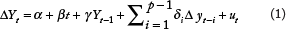
Where t is the time index, Yt is the value of time series at time t, ∆Yt denotes the lagged first differences (i.e., Yt – Yt-1). α is an intercept constant (a drift term), β is a coefficient on a time trend and γ is a coefficient to test whether we need to difference the data to make it stationary. P is the lag length of the test and determined when applying the test. The Akaike Information Criterion (AIC) is used to identify the lag lengths. It is an independent identically distributed residual term. The null hypothesis of the test is that the time series under study is not stationary (γ = 0, β ≠ 0), and the alternative hypothesis is that the time series is stationary (γ < 0, β ≠ 0).
GRANGER CAUSALITY TEST
The Granger causality test (Granger, 1969) is a statistical hypothesis test to determine whether the time series of a variable is useful to predict the time series of another variable. In other words, this test determines whether the time series of a variable leads the time series of another variable. The null hypothesis of this test is that the past P values of X are not helpful to predict Y (X does not Granger cause Y). P is the lag length of the Granger causality test, and the results of the test depend on the chosen lag lengths. Therefore, different lag lengths (1, 2, 3, 4, 5, 6, 7, 8, 9, 10 lag lengths) are used in this study. These lag lengths represent a 2.5-year horizon since the data are quarterly. The following bivariate autoregressive models are used to test whether the value added by construction Granger causes GDP at the state level and vice versa (GDP Granger causes CVA):


Where CVA(t) represents the time series of the Construction Value Added in the state, GDP(t) is the time series of Gross Domestic Product in the same state, P is the maximum number of lagged observations included in the model, and ut represents the time series of the residuals. CVA does not Granger cause GDP if βi = 0 (i=1,…,P) in Equation 2. GDP does not Granger cause CVA if βi = 0 (i=1,…,P) in Equation 3.
COINTEGRATION TEST
Two-time series variables are cointegrated if the time series variables are integrated in the same order and a linear combination of these two-time series has a lower order of integration. If a combination of two variables is cointegrated, they do not drift apart as time passes and they are related in the long run.
In this paper, a cointegration test proposed by Johansen (1988) and extended by Johansen and Juselius (1990) was implemented to examine whether CVA is cointegrated with GDP in each state of the U.S. The lag length (p) for this test was selected based on Akaike Information Criterion (Akaike, 1974). r represents the number of cointegrating relationships between GDP and CVA. The trace statistics show that whether the null hypothesis of r = 0 could be rejected. If the null hypothesis is rejected, there is a cointegrating relationship (or are relationships) between GDP and CVA at the state level.
Data
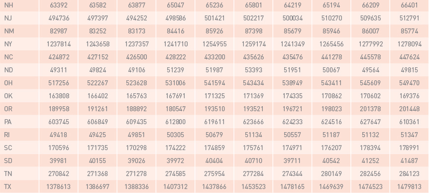
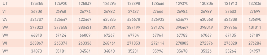
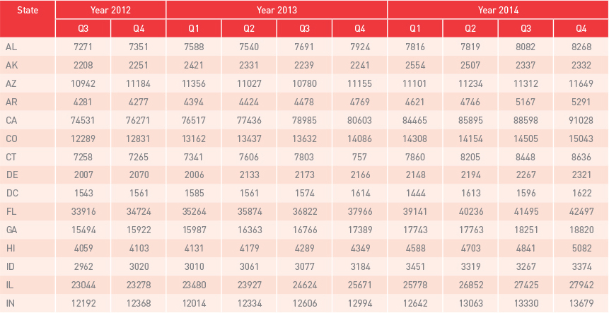
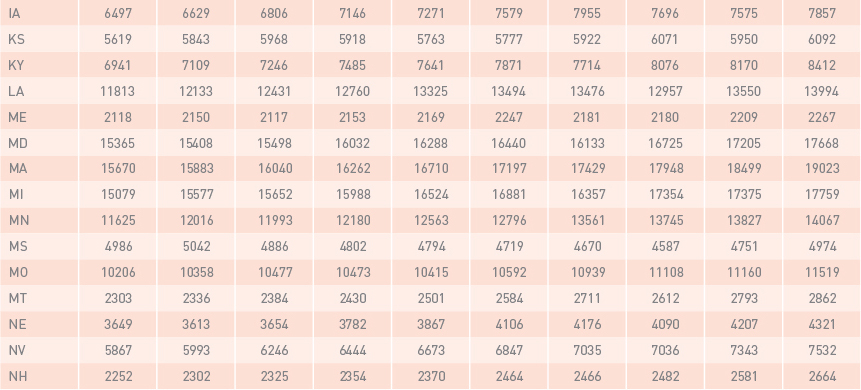
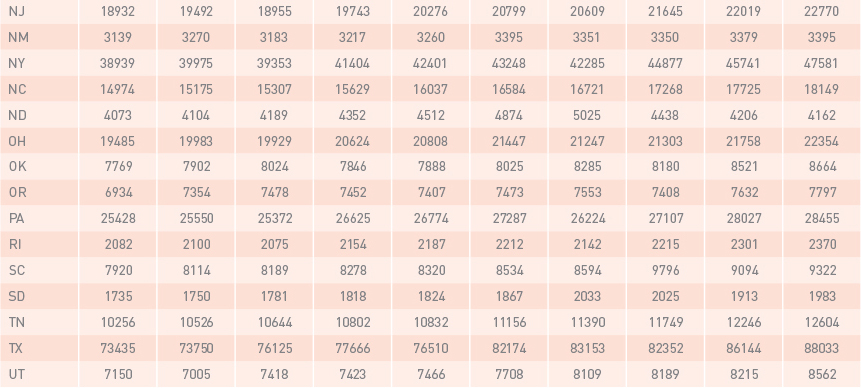
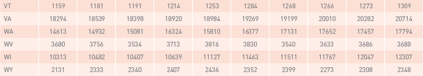
Non-seasonally adjusted quarterly data of real GDP and CVA published by the Bureau of Economic Analysis (BEA, 2016) was used in this study. Real Gross Domestic product (real GDP) is a monetary measure of final goods and services. This measure has been widely used for economic analyses. The Bureau of Economic Analysis (BEA) has published “quarterly real GDP by state” since 2005. The contribution of each industry to the overall GDP by state is called value added by the industry. In concept, value added of an industry is equivalent to the industry’s gross output minus its intermediate inputs (Strassner and Wasshausen, 2014). Construction Value Added (CVA) represents the contribution of the construction industry to the GDP by state. It includes the value added by several construction activities, such as construction of highways and streets, manufacturing structures, health care structures, educational and vocational structures, and residential structures. As an illustration, Table 6 and Table 7, in appendix A, represent GDPs and CVAs for all U.S. states and the District of Columbia from the 3rd quarter of 2012 up to the 4th quarter of 2014.
Empirical results
The results of ADF unit root tests for the state GDPs and CVAs are represented in Table 1. Data of GDPs for the states are not stationary first. The GDPs of 47 states and the District of Columbia become stationary by applying the differencing operator once (∆GDP). These results also show that the CVAs of 38 states and the District of Columbia become stationary after applying the differencing operator ∆CVA.
| State | ADF t-statistics for ∆GDP | ADF t-statistics for ∆CVA |
|---|---|---|
| AK | -3.73** | -4.55*** |
| AL | -4.61*** | -3.33* |
| AR | -4.59*** | -5.37*** |
| AZ | -2.55 | -2.43 |
| CA | -4.16** | -7.39*** |
| CO | -4.49*** | -3.54** |
| CT | -3.86** | -3.73** |
| DC | -4.57*** | -4.67*** |
| DE | -5.25*** | -5.16*** |
| FL | -2.32 | -2.14 |
| GA | -3.95** | -2.29 |
| HI | -3.59** | -1.98 |
| IA | -4.62*** | -5.08*** |
| ID | -3.59** | -4.26*** |
| IL | -4.16** | -2.87 |
| IN | -3.49* | -3.71** |
| KS | -4.06** | -4.52*** |
| KY | -3.82** | -4.86*** |
| LA | -4.21** | -4.73*** |
| MA | -4.05** | -2.64 |
| MD | -4.79*** | -4.19** |
| ME | -5.18*** | -4.42*** |
| MI | -3.26* | -4.23*** |
| MN | -4.77*** | -3.99** |
| MO | -5.2*** | -3.74** |
| MS | -3.92** | -3.99** |
| MT | -3.96** | -3.64** |
| NC | -4.13** | -2.72 |
| ND | -3.16 | -3.71** |
| NE | -5.66*** | -4.95*** |
| NH | -6.34*** | -4.58*** |
| NJ | -3.47* | -4.64*** |
| NM | -5.57*** | -2.78 |
| NV | -2.75 | -2.16 |
| NY | -5.15*** | -4.07** |
| OH | -3.96** | -3.74** |
| OK | -5.24*** | -4.84*** |
| OR | -3.94** | -2.63 |
| PA | -5.84*** | -4.43*** |
| RI | -4.47*** | -3.6** |
| SC | -3.82** | -2.56 |
| SD | -3.69** | -5.36*** |
| TN | -3.93** | -3.87** |
| TX | -4.1** | -3.61** |
| UT | -4.13** | -2.1 |
| VA | -5.48*** | -4.21** |
| VT | -4.99*** | -5.53*** |
| WA | -3.72** | -2.16 |
| WI | -5.15** | -5.39*** |
| WV | -5.18*** | -4.92*** |
| WY | -4.48*** | -4.7*** |
| Notes: *, **, and *** represent rejection of null hypothesis at the 10%, 5%, and 1% significance levels, respectively. Akaike Information Criterion is used for lag selection. | ||
To avoid the problem of spurious regression, the Granger causality test can only be applied on stationary time series data. Both CVAs and GDPs of 36 states and District of Columbia become stationary after applying the difference operator once. Therefore, the Granger causality test was applied on CVAs and GDPs of 36 states and the District of Columbia in which CVAs and GDPs become stationary after applying the differencing operator once. The Granger causality test investigates whether the first differenced time series of CVA of a specific state Granger causes the first differenced time series of GDP in the same state.
The results of Granger causality tests summarized in Table 2 indicate that CVA is a leading indicator of GDP in 18 states (Alaska, California, Colorado, Connecticut, Delaware, Idaho, Indiana, Louisiana, Minnesota, Missouri, Montana, New Hampshire, New Jersey, New York, Oklahoma, Wisconsin, West Virginia, Wyoming) and the District of Columbia.
| State | F Statistics | |||||||||
|---|---|---|---|---|---|---|---|---|---|---|
| Lag 1 | Lag 2 | Lag 3 | Lag 4 | Lag 5 | Lag 6 | Lag 7 | Lag 8 | Lag 9 | Lag 10 | |
| AK | 2.39 | 1.98 | 2.33* | 1.59 | 1.36 | 1.28 | 0.89 | 0.71 | 0.77 | 0.62 |
| CA | 8.53*** | 4.55** | 2.35* | 1.66 | 2.16* | 2.33* | 1.95 | 2 | 1.64 | 1.14 |
| CO | 3.48* | 2.8* | 2.14 | 1.86 | 1.32 | 2.43* | 1.58 | 2.3* | 1.53 | 1.25 |
| CT | 1.24 | 1.74 | 1.36 | 1.23 | 3.18** | 2.7** | 2.33* | 3.53** | 3.91*** | 6.4*** |
| DC | 0.47 | 0.83 | 1.03 | 3.08** | 3.2** | 1.54 | 1.16 | 1.19 | 0.77 | 0.61 |
| DE | 1.72 | 1.93 | 3.1** | 2.16 | 1.79 | 1.58 | 1.14 | 1.13 | 1.17 | 1.22 |
| ID | 0.59 | 1.28 | 4.72*** | 3.38** | 4.21*** | 4.16*** | 3.45** | 3.2** | 2.36* | 2.06 |
| IN | 3.94* | 1.99 | 0.87 | 0.67 | 0.59 | 0.53 | 0.49 | 0.54 | 0.51 | 0.46 |
| LA | 2.41 | 2.89* | 2.27* | 1.84 | 1.41 | 0.98 | 1.16 | 1.97 | 1.45 | 1.05 |
| MN | 3.55* | 2.36 | 2.64* | 2 | 1.2 | 1.09 | 1.8 | 2.85** | 2.04 | 1.82 |
| MO | 1.04 | 0.68 | 0.58 | 1.39 | 1.89 | 1.52 | 1.93 | 2.02* | 1.5 | 0.81 |
| MT | 3.29* | 2.13 | 0.91 | 0.94 | 0.86 | 0.59 | 1.03 | 1.87 | 1.81 | 2.19* |
| NH | 0.94 | 2.25 | 3.25** | 3.46** | 3.29** | 3.71*** | 2.44* | 1.65 | 2.27* | 1.87 |
| NJ | 0.06 | 0.99 | 0.91 | 2.58* | 2.61** | 2.78** | 2.29* | 1.69 | 2.16* | 1.67 |
| NY | 4.31** | 2.04 | 1.51 | 0.93 | 1.21 | 0.87 | 1.07 | 1.3 | 0.91 | 0.98 |
| OK | 2.81 | 1.24 | 0.65 | 2.06 | 2.65** | 2.3* | 1.91 | 2 | 1.7 | 1.57 |
| WI | 1.03 | 0.92 | 1.43 | 1.05 | 0.84 | 1.18 | 2.34* | 2.56** | 2.83** | 2.27* |
| WV | 0.32 | 0.45 | 2.28* | 1.86 | 1.47 | 1.49 | 1.44 | 1.32 | 0.89 | 0.75 |
| WY | 0.0001 | 0.001 | 1.69 | 4.85*** | 4.13*** | 3** | 2.74** | 2.41* | 2.29* | 1.82 |
| Notes: *, **, and *** represent rejection of null hypothesis at the 10%, 5%, and 1% significance levels, respectively. | ||||||||||
Figure 1 demonstrates the geographic distribution of the states where CVA leads GDP. These states do not belong to a specific geographical area.
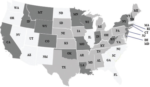
Figure 1 Granger causality map between CVA and GDP
| Value added by construction industry leads GDP by state | 18 states |
| Value added by construction industry does not lead GDP by state | 18 states |
| Granger causality test could not be tested | 14 states |
Granger causality test is also applied to understand whether GDP is a leading indicator of CVA at the state level. Rejection of null hypothesis (GDP does not Granger cause CVA at the state level) for time series data of a state means that the Granger causality runs from GDP to CVA at that state. Table 3 shows the states in which GDP Granger causes CVA. The results indicate that in 10 states (Colorado, Delaware, Iowa, Kansas, Louisiana, Michigan, Montana, Minnesota, Nebraska, and Rhode Island) and the District of Columbia causality runs from GDP to CVA, which means CVA is a lagging indicator of GDP in these states.
| State | F Statistics | |||||||||
|---|---|---|---|---|---|---|---|---|---|---|
| Lag 1 | Lag 2 | Lag 3 | Lag 4 | Lag 5 | Lag 6 | Lag 7 | Lag 8 | Lag 9 | Lag 10 | |
| CO | 4.98** | 2.70* | 2.98** | 2.03 | 1.88 | 3.21** | 2.51** | 1.77 | 1.58 | 1.16 |
| DC | 3.77* | 2.26 | 0.96 | 3.79** | 2.99** | 2.96** | 2.37* | 2.25* | 2.02 | 1.77 |
| DE | 16.9*** | 7.91*** | 5.16*** | 0.33 | 0.41 | 0.87 | 1.35 | 1.04 | 0.78 | 0.71 |
| IA | 0.29 | 4.37** | 2.70* | 2.53* | 2.32* | 1.74 | 1.38 | 1.46 | 1.17 | 1.30 |
| KS | 0.007 | 1.41 | 0.86 | 0.59 | 0.58 | 0.45 | 0.90 | 0.74 | 2.09* | 2.29* |
| LA | 0.29 | 4.37** | 2.70* | 2.53* | 2.32* | 1.74 | 1.38 | 1.46 | 1.17 | 1.30 |
| MI | 2.79 | 3.69** | 2.41* | 1.99 | 1.44 | 2.43* | 2.06* | 1.79 | 1.47 | 1.32 |
| MO | 0.96 | 0.54 | 1.53 | 1.62 | 2.39* | 1.78 | 1.21 | 1.09 | 1.03 | 1.13 |
| MT | 0.09 | 1.21 | 1.27 | 3.47** | 3.51** | 2.90** | 2.37* | 1.62 | 1.40 | 1.79 |
| NE | 0.45 | 0.30 | 1.31 | 2.21 | 2.08* | 1.73 | 1.65 | 1.34 | 1.01 | 0.69 |
| RI | 0.38 | 0.96 | 1.87 | 2.09 | 3.00** | 3.04** | 3.09** | 2.64** | 3.41** | 3.26** |
| Notes: *, **, and *** represent rejection of null hypothesis at the 10%, 5%, and 1% significance levels, respectively. | ||||||||||
Johansen Cointegration test is also applied on time series data of the states in which either CVA Granger causes GDP or GDP Granger causes CVA. As discussed earlier, time series data of these states are integrated of order 1. If CVA and GDP time series data of a state are both integrated of order 1 and a linear combination of GDP and CVA is integrated of order 0, these two-time series data are cointegrated. Rejection of null hypothesis (r =0) in cointegration test at each state means that there exists a long-run relationship between GDP and CVA at the state level. The results of cointegration test summarized in Table 4 show that there is a statistically significant cointegrating relationship between GDP and CVA in 8 states of the U.S. (Connecticut, Idaho, Michigan, Montana, New Hampshire, New Jersey, Rhode Island, and Wisconsin) and the District of Columbia.
| State | Trace statistics | 5% critical value | 1% critical value |
|---|---|---|---|
| CT | 23.85*** | 17.95 | 23.52 |
| DC | 31.22*** | 17.95 | 23.52 |
| ID | 22.34** | 17.95 | 23.52 |
| MI | 27.51*** | 17.95 | 23.52 |
| MT | 33.22*** | 17.95 | 23.52 |
| NH | 18.03** | 17.95 | 23.52 |
| NJ | 26.96*** | 17.95 | 23.52 |
| RI | 24.32*** | 17.95 | 23.52 |
| WI | 31.37*** | 17.95 | 23.52 |
| Notes: **, and *** represent rejection of null hypothesis at the 5%, and 1% significance levels, respectively; Akai Information Criterion is used for lag selection. | |||
Discussion of results
The results of this study show that out of 36 states in which the temporal relationship between GDP and CVA could be empirically tested, there exists a leading and/or lagging relationship between the construction industry and GDP in 23 states. CVA is a leading indicator of GDP in 18 states and the District of Columbia; CVA is a lagging indicator of GDP in 10 states and the District of Columbia, and there is a bi-directional relationship between CVA and GDP in 5 states and the District of Columbia. We did not find enough evidence showing any causality relationships between CVA and GDP in the other 13 states; however, it does not necessarily mean that the construction industry is not important in these states. The results of this study are summarized in Table 5.
STATES IN WHICH CVA IS A LEADING INDICATOR OF GDP
The results of this study show that CVA is a leading indicator of GDP in 18 states and the District of Columbia. CVA leads GDP in the short-term in 7 states (AK, CA, DE, IN, LA, NY, WV) and the District of Columbia. CVA leads GDP in the medium- to long-term in 5 states (CT, NJ, OK, WI, WY). CVA leads GDP in both short and medium to long-term in 6 states (CO, ID, MN, MO, MT, NH); therefore, construction activity is the consistent leading indicator of economic growth in these states.
STATES IN WHICH CVA IS A LAGGING INDICATOR OF GDP
The results of the Granger causality test from GDP to CVA show that CVA is a lagging indicator of GDP in 10 states and the District of Columbia that means changes in GDP would take place before a change in the construction sector. Economic variations in some states take place right before the construction sector (DE, IA, LA) while in some other states (KS, MO, MT, NE, RI) these variations will show up in the construction industry up to 2.5 years later. GDP Granger causes CVA in both the short and medium to long-term in two states (CO, MI) and the District of Columbia. These results confirm the dependency of the construction sector to the economic conditions in these 10 states and the District of Columbia.
STATES IN WHICH CVA IS A LEAD-LAG INDICATOR OF GDP
There exists a bi-directional causal relationship between CVA and GDP in 5 states (CO, DE, LA, MO, MT) and the District of Columbia that means while changes in the economic conditions of the state will appear later in the construction sector, construction activities are still an engine of economic variations in these states.
STATES IN WHICH CVA AND GDP ARE COINTEGRATED
The data of CVA and GDP are cointegrated in 8 states (CT, ID, MI, MT, NH, NJ, RI, WI) and the District of Columbia. The cointegration relationship means that the time series of the two variables do not drift apart as time passes and there is a long-run relationship between CVA and GDP in these states.
THE ASSOCIATION BETWEEN LEADING/LAGGING RELATIONSHIPS AND SHARE OF CVA IN GDP
The Bureau of Economic Analysis calculates the share of construction activity in the state GDP. North Dakota, Montana, Wyoming, Louisiana, and Utah are the top 5 states with respect to the share of construction activity in the state GDP in 2015 (BEA, 2016). New York, Connecticut, Delaware, Oregon, and Ohio are the bottom 5 states in this ranking (BEA, 2016). Some of the 18 states shown in Table 1 are among the states with high share of construction activity in the GDP. For example, Montana, Wyoming, and Louisiana are ranked among the top 5 states of the ranking table of construction activity as a percentage of state GDP. On the contrary, some other states of Table 1 are among the bottom 5 states of this ranking (New York, Connecticut, and Delaware). Thus, the hypothesis of an existing relationship between the “share of construction in state GDP” and the “impact of construction industry on state GDP” in all U.S. states would be rejected. In other words, a higher share of construction to the state GDP does not necessarily mean that construction investments have more impact on the state’s economy. More interestingly, a lower share of construction to the state GDP does not necessarily indicate the low importance of construction in economic growth of the state.
Conclusion
This study analyzes the temporal relationships between the construction industry and the economy at the state level in the U.S. The results of the present study show that the value added by the construction industry leads state GDP with different lags in 18 states of the U.S. (Alaska, California, Colorado, Connecticut, Delaware, Idaho, Indiana, Louisiana, Minnesota, Missouri, Montana, New Hampshire, New Jersey, New York, Oklahoma, Wisconsin, West Virginia, Wyoming) and the District of Columbia. Since growth in the construction industry precedes growth in the larger economy in 18 states and the District of Columbia, the government had better provide a conductive requirement for construction firms at least in these states, to enhance their performance. This finding could be useful in policy planning while prioritizing investment opportunities.
The results of this study also show that CVA is a lagging indicator of GDP in 10 states (Colorado, Delaware, Iowa, Kansas, Louisiana, Michigan, Minnesota, Montana, Nebraska, and Rhode Island) and the District of Columbia that means changes in economic conditions will appear later in the construction sector in these states. Economic variations in some states take place right before changes in the construction industry such as in Delaware while in some other states (e.g. Rhode Island) these variations will show up in the construction industry up to 2.5 years later. Correspondingly, there is a bi-directional causal relationship between CVA and GDP in 5 states (Colorado, Delaware, Louisiana, Minnesota, and Montana) and the District of Columbia that shows the dependency of the construction sector and the economy on each other in these states.
We did not find enough evidence showing any relationships between the Value Added by Construction industry and state GDP in other states. The data of 14 states were not stationary; therefore, the Granger causality test could not be conducted. This limitation of the study should not be interpreted as minor importance of the construction industry in those states.
A comparison between the results of this study and the table of construction as a percentage of GDP shows that the hypothesis of an existing relationship between the “share of construction in state GDP” and the “impact of construction industry on state GDP” in all U.S. states would be rejected. In other words, a higher share of construction to the state GDP does not necessarily mean that construction investments have more impact on the state’s economy. More interestingly, a lower share of construction to the state GDP does not necessarily mean the low importance of construction in economic growth of the state. It is recommended to further investigate the relationships between state GDP growth rates and construction share of GDP. Further studies could also be conducted analyzing the impact of investments in different sub-sectors of the construction industry on the economy of the U.S. states.
DECLARATION OF CONFLICTING INTEREST The author(s) declared no potential conflicts of interest with respect to the research, authorship, and/or publication of this article. FUNDING The author(s) received no financial support for the research, authorship, and/or publication of this article.
References
Appendix A